![]()
Welcome to the Light Dark Matter eXperiment! This is the central page for documenting our software. Here, you will find manually written documents as well as links to other manuals related to the software. This site is generated using mdbook which has a helpful page on how to read a site formatted like this. All of the pages are hosted here except for the pages in the Reference section which are links to the manuals hosted at different sites.
Below is a list of past video tutorials that are available online. Some of them may be out of date, but they can still be helpful in defining what kind of vocabulary we often use. The first section of this manual is text-based information about how to get started using (and eventually developing) ldmx-sw.
- ldmx-sw v2.0.0 tutorial May 2020
- ldmx-sw v3.0.0 tutorials (links to session recordings included)
This manual is separated into two main sections based on how you are interacting with ldmx-sw.
- Using is when you are running ldmx-sw with fire and are not actively changing code within ldmx-sw (i.e. you can fix the version of ldmx-sw you are using for your work).
- Developing is when you are actively changing code within ldmx-sw and so need to compile ldmx-sw yourself.
Notice that this categorization only cares about the ldmx-sw source code. People using ldmx-sw very often are still developing code that may just not be within ldmx-sw. Additionally, whether or not you are developing ldmx-sw may change depending on the project you are working on. Perhaps you find a bug or think of a new feature -- contributions are encouraged and welcome!
Getting Started
This guide is focused on first-time users of ldmx-sw. If you are interested in contributing to ldmx-sw, please look at the getting started developing guide for help starting to develop ldmx-sw.
ldmx-sw is a large software project that builds on top of other large and complicated software projects. For this reason, we have chosen to use containers to share fixed software environments allowing all of us to know exactly what version of ldmx-sw (and its underlying packages) is being used.
Each of the steps below is really short but more detail has been added in order to help users debug any issues they may encounter. If all goes well, you will be able to fly through these instructions within 5-10 minutes (depending on how long software installations take). Each of the sections has a "Comments" subsection for extra details and a "Test" subsection allowing you to verify that you completed that step successfully.
While many new ldmx-sw users may be unfamiliar with the terminal, explaining its use is beyond the scope of this site. If you are unfamiliar with the terminal, a helpful resource is linuxcommand.org and there are many others available online since terminals are a common tool utilized by software developers.
Windows Comments
- If you are running on a Microsoft Windows system, it is necessary for you to do all of the steps below within Windows Subsystem for Linux (WSL). The permissions system that docker relies on in order to effectively run the containers is not supported by Windoze. (While GitBash and the Command Prompt can look similar to other terminals, make sure to open a WSL terminal --- often labeled "Ubuntu").
- As of this writing, you cannot use a VPN and connect to the internet from within WSL
- The "docker daemon" needs to be running. On most systems, this program starts automatically when the computer is booted. You can check if the docker daemon is running by trying to run a simple docker container. If it is not running, you will need to start it manually.
- Docker Desktop outside WSL needs to be running to be able to use docker inside WSL? (question mark because unsure)
Install a Container Runner
Currently, we use denv to help shorten and unify container interaction across
a few different runners, so we only require a container runner supported by denv.
On personal laptops, most users will find it easiest to install the docker engine.
apptainer should already be installed on shared computing clusters.1
- If you are on Windows, make sure to use the WSL2 backend for docker.
- On Linux systems, make sure to manage docker as non-root user
so that you can run that command without
sudo. - If you choose to use
podman, make sure to update theregistries.confconfiguration file in order to allow forpodmanto pull from DockerHub.
You can run a simple container in whichever runner is available.
docker run hello-world
or
apptainer run docker://ghcr.io/apptainer/lolcow
This may be the first point where you enter into a terminal unless your installation was terminal-based. If you are using Windows, remember to go into Windows Subsystem for Linux rather than other Windows terminals like GitBash or Command Prompt.
For those who've been using containers (with or without LDMX) for awhile,
the program singularity may sound familiar.
apptainer is just a new brand name for singularity after it was adopted
by the Linux foundation.
Many apptainer installations also come with a wrapper program
called singularity for backwards compatibility.
Install denv
For most users the following command will install the latest version of denv
curl -s https://raw.githubusercontent.com/tomeichlersmith/denv/main/install | sh
If it doesn't work follow these instructions for installing denv.
They are short but require you to be in the terminal.
- Remember to install
denvwithin WSL if you are using Windows. - While
denv's install script tries to help you update yourPATHvariable, it may not be perfect. You may need to consult the documentation for your shell on how to add new directories to thePATHvariable so that thedenvcommand can be found by your shell.
Replicating the Legacy ldmx Command
Replicating the Legacy ldmx Command
Some folks want to replicate the ldmx bash function which preceeded denv.
To do this, you can create a few symlinks.
The examples below are for the default installation prefix for denv
(~/.local), but you can replace this directory with whereever you chose
to install denv when running the curl ... install command.
# for the command
ln -s ~/.local/bin/denv ~/.local/bin/ldmx
# and for the tab completion
ln -s ~/.local/share/bash-completion/completions/denv \
  ~/.local/share/bash-completion/completions/ldmx
You should be able to have denv run its self-check that also
ensures you have a supported container runner installed.
denv check
Example output would look like
Entrypoint found alongside denv
Looking for apptainer... not found
Looking for singularity... not found
Looking for podman... not found
Looking for docker... found 'Docker version 27.0.3, build 7d4bcd8' <- use without DENV_RUNNER defined
denv would run with 'docker'
Set Up Workspace
Whatever your project is, it will be helpful to have a directory on your computer that holds the files related to this project. If you haven't already made a directory for this purpose, now is the time! This is also where we will choose the version of ldmx-sw to use.
# create a directory for the project
mkdir -p ldmx/my-project
# go into that directory
cd ldmx/my-project
# initialize a new denv, defining the ldmx-sw version
denv init ldmx/pro:v4.0.1
- The specific location of the
my-projectdirectory does not matter. (As long as its within WSL if you're on Windows of course!) - The version of ldmx-sw listed here is just an example, changing the version later can be done with
denv config image ldmx/pro:<ldmx-sw-version>if desired.
The denv init command should not be run from within ldmx-sw.
This could lead to a confusing state where the fire being run
is not the one associated with the ldmx-sw that resides in that
directory.
We can make sure you have access to ldmx-sw by trying to have ldmx-sw's core program fire
printout its help message.
denv fire
This should look something like
$ denv fire
Usage: fire {configuration_script.py} [arguments to configuration script]
     configuration_script.py  (required) python script to configure the processing
     arguments                (optional) passed to configuration script when run in python
Using Legacy Versions of ldmx-sw
Using Legacy Versions of ldmx-sw
Versions of ldmx-sw that were built with a version of the development image before 4.2.2 (generaly pre-v4 ldmx-sw) do not have some ease-of-use updates to enable running ldmx-sw from within a denv.
One can still use a denv without much effort. In short, you must update the denv shell's profile.
denv exit 0 # make sure a template .profile is created
Add the following lines to the end of .profile that is in your working
directory (not the .profile in your home directory if you have one).
# add ldmx-sw and ldmx-analysis installs to the various paths
# LDMX_SW_INSTALL is defined when building the production image or users
# can use it to specify a non-normal install location
if [ -z "${LDMX_SW_INSTALL+x}" ]; then
  if [ -z "${LDMX_BASE+x}" ]; then
    printf "[ldmx-env-init.sh] WARNING: %s\n" \
      "Neither LDMX_BASE nor LDMX_SW_INSTALL is defined." \
      "At least one needs to be defined to ensure a working installation."
  fi
  export LDMX_SW_INSTALL="${LDMX_BASE}/ldmx-sw/install"
fi
export LD_LIBRARY_PATH="${LDMX_SW_INSTALL}/lib:${LD_LIBRARY_PATH}"
export PYTHONPATH="${LDMX_SW_INSTALL}/python:${LDMX_SW_INSTALL}/lib:${PYTHONPATH}"
export PATH="${LDMX_SW_INSTALL}/bin:${PATH}"
This is just a short term solution and needs to be done on every computer. Updating to more recent ldmx-sw is advised.
Running a Configuration Script
The next step now that you have access to fire is to run a specific configuration
of ldmx-sw with it!
Configuration scripts are complicated in their own right and have
been given their own chapter.
The next chapter is focused on analyzing event files that have been shared with you
(or generated with a config shared with you) since, generally, analyzing events is
done before development of the configs that produce those events.
Analyzing ldmx-sw Event Files
Often when first starting on LDMX, people are given a .root file produced by ldmx-sw
(or some method for producing their own file). This then leads to the very next
and reasonable question -- how to analyze the data in this file?
Many answers to this question have been said and many of them are functional. In subsequent sections of this chapter of the website, I choose to focus on highlighting two possible analysis workflows that I personally like (for different reasons).
I am not able to fully cover all of the possible different types of analysis, so I am writing this guide in the context of one of the most common analyses: looking at a histogram. This type of analysis can be broken into four steps.
- Load data: from a data file, load the information in that file into memory.
- Data Manipulation: from the data already present, calculate the variable that you would like to put into the histogram.
- Histogram Filling: define how the histogram should be binned and fill the histogram with the variable that you calculated.
- Plotting: from the definition of the histogram and its content, draw the histogram in a visual manner for inspection.
The software that is used to do each of these steps is what mainly separates the different analysis workflows, so I am first going to mention various software tools that are helpful for one or more of these steps. I have separated these tools into two "ecosystems", both of which are popularly used within HEP.
| Purpose | ROOT | scikit-hep |
|---|---|---|
| Load Data | TFile,TTree | uproot |
| Manipulate Data | C++ Code | Vectorized Python with awkward |
| Fill Histograms | TH1* | hist,boost_histogram |
| Plot Histograms | TBrowser, TCanvas | matplotlib,mplhep |
How one mixes and matches these tools is a personal choice, especially since the LDMX collaboration has not landed on a widely agreed-upon method for analysis. With this in mind, I find it important to emphasize that the following subsections are examples of analysis workflows -- a specific analyzer can choose to mix and match the tools however they like.
Caveat
While I (Tom Eichlersmith) have focused on two potential analysis workflows, I do not mean to claim that I have tried all of them and these two are "the best". I just mean to say that I have drifted to these two analysis workflows over time as I've looked for easier and better methods of analyzing data. If you have an analysis workflow that you would like to share, add another subsection to this chapter of the website!
Using Python (Efficiently)
Python is slow. I can't deny it. But Python, for better or for worse, has taken over the scientific programming ecosystem meaning there are a large set of packages that are open source, professionally maintained, and perform the common tasks that scientists want to do.
One aspect of Python that has enabled its widespread adoption
(I think) is the relative ease of writing packages in another
programming language. This means that most of our analysis
code will not be using "pure Python", but instead be using
compiled languages (C++ mostly) hidden behind some convenience
wrappers. This is the strategy of many popular Python packages
numpy, scipy, and the HEP-specific hist and awkward.
My biggest tip for any new Python analyzers is to avoid writing
the for loop. As mentioned, Python itself is slow, so only
write for if you know you are only looping over a small number
of things (e.g. looping over the five different plots you want
to make). We can avoid for by using these packages with compiled
languages under-the-hood. The syntax of writing these "vectorized"
operations is often complicated to grasp, but it is concise, precise,
and performant.
With those introductory ramblings out of the way, let's get started.
Set Up
The packages we use (and the python ecosystem in general) evolves relatively fast. For this reason, it will be helpful to use a newer python version such that you can access the newer versions of the packages. Personally, I use denv to pick new python without needing to compile it and then have my installed packages for that python be isolated to within my working directory.
While you can install the packages I'll be using directly, they (and a few other helpful
ones) are availabe withing the scikit-hep metapackage allowing a quick and simple
installation command. In addition, Jupyter Lab offers an excellent way to see
plots while your constructing them and recieve other feedback from your code in an
immediate way (via a REPL
for those interested).
cd work-area
denv init python:3.11
denv pip install scikit-hep jupyterlab
In addition, you will need some data to play with. I generated the input events.root
file using an ldmx-sw simulation, but I am using common event objects that exist in
most (if not all) event files, so this example should work with others.
Generate Event File with ldmx-sw
Generate Event File with ldmx-sw
Again, I used denv to pin the ldmx-sw version and generate the data file.
denv init ldmx/pro:v3.3.6 eg-gen
cd eg-gen
denv fire config.py
mv events.root path/to/work-area/
where config.py is the following python configuration script.
from LDMX.Framework import ldmxcfg
p = ldmxcfg.Process('test')
from LDMX.SimCore import simulator as sim
mySim = sim.Simulator( "mySim" )
mySim.set_detector( 'ldmx-det-v15-8gev', True )
from LDMX.SimCore import generators as gen
mySim.generators = [ gen.single_8gev_e_upstream_tagger() ]
mySim.description = 'Basic test Simulation'
p.sequence = [ mySim ]
p.run = 1
p.max_events = 10000
p.output_files = [ 'events.root' ]

import LDMX.Ecal.ecal_geometry
import LDMX.Ecal.ecal_hardcoded_conditions
import LDMX.Hcal.hcal_geometry
import LDMX.Ecal.digi as ecal_digi

p.sequence = [
    mySim,
    ecal_digi.EcalDigiProducer(),
    ecal_digi.EcalRecProducer()
]
Launch a jupyter lab with
denv jupyter lab
open the link in your browser and create a new notebook to get started.
Notebooks consist of "cells" which
can contain "markdown" (a way to write write formatted text), code that will be executed, and raw text.
The rest of these sections are the the result of exporting a jupyter notebook (a *.ipynb file)
into "markdown" and then including it in this documentation here.
# load the python modules we will use
import uproot # for data loading
import awkward as ak # for data manipulation
import hist # for histogram filling (and some plotting)

import matplotlib as mpl # for plotting
import matplotlib.pyplot as plt # common shorthand
import mplhep # style of plots
%matplotlib inline
mpl.style.use(mplhep.style.ROOT) # set the plot style
Load Data
The first step to any analysis is loading the data.
For this step in this analysis workflow, we are going to use the uproot package
to load the data into awkward arrays in memory.
Some helpful links to find more details on this
%%time
# while the uproot file is open, conver the 'LDMX_Events' tree into in-memory arrays
with uproot.open('events.root') as f:
    events = f['LDMX_Events'].arrays()
# show the events array
events
CPU times: user 3.63 s, sys: 220 ms, total: 3.85 s
Wall time: 3.85 s
Printout of `events` array
[{'SimParticles_test.first': [1, 2, 3, ..., 48, 49], ...},
 {'SimParticles_test.first': [1, 2, 3, ..., 61, 62], ...},
 {'SimParticles_test.first': [1, 2, 3, ..., 11, 12], ...},
 {'SimParticles_test.first': [1, 2, ..., 15, 1199], ...},
 {'SimParticles_test.first': [1, 2, 3, ..., 8, 9], ...},
 {'SimParticles_test.first': [1, 2, ..., 118, 119], ...},
 {'SimParticles_test.first': [1, 2, 3, ..., 10, 11], ...},
 {'SimParticles_test.first': [1, 2, 3, ..., 10, 11], ...},
 {'SimParticles_test.first': [1, 2, 3, ..., 7, 61], ...},
 {'SimParticles_test.first': [1, 2, 3, ..., 10, 11], ...},
 ...,
 {'SimParticles_test.first': [1, 2, 3, ..., 9, 10], ...},
 {'SimParticles_test.first': [1, 2, ..., 126, 127], ...},
 {'SimParticles_test.first': [1, 2, 3, ..., 9, 10], ...},
 {'SimParticles_test.first': [1, 2, ..., 85, 4702], ...},
 {'SimParticles_test.first': [1, 2, ..., 72, 6976], ...},
 {'SimParticles_test.first': [1, 2, 3, ..., 8, 93], ...},
 {'SimParticles_test.first': [1, 2, ..., 7120], ...},
 {'SimParticles_test.first': [1, 2, ..., 7921], ...},
 {'SimParticles_test.first': [1, 2, 3, ..., 8, 9], ...}]
---------------------------------------------------------------------
type: 10000 * {
    "SimParticles_test.first": var * int32,
    "SimParticles_test.second.energy_": var * float64,
    "SimParticles_test.second.pdgID_": var * int32,
    "SimParticles_test.second.genStatus_": var * int32,
    "SimParticles_test.second.time_": var * float64,
    "SimParticles_test.second.x_": var * float64,
    "SimParticles_test.second.y_": var * float64,
    "SimParticles_test.second.z_": var * float64,
    "SimParticles_test.second.endX_": var * float64,
    "SimParticles_test.second.endY_": var * float64,
    "SimParticles_test.second.endZ_": var * float64,
    "SimParticles_test.second.px_": var * float64,
    "SimParticles_test.second.py_": var * float64,
    "SimParticles_test.second.pz_": var * float64,
    "SimParticles_test.second.endpx_": var * float64,
    "SimParticles_test.second.endpy_": var * float64,
    "SimParticles_test.second.endpz_": var * float64,
    "SimParticles_test.second.mass_": var * float64,
    "SimParticles_test.second.charge_": var * float64,
    "SimParticles_test.second.daughters_": var * var * int32,
    "SimParticles_test.second.parents_": var * var * int32,
    "SimParticles_test.second.processType_": var * int32,
    "SimParticles_test.second.vertexVolume_": var * string,
    "TaggerSimHits_test.id_": var * int32,
    "TaggerSimHits_test.layerID_": var * int32,
    "TaggerSimHits_test.moduleID_": var * int32,
    "TaggerSimHits_test.edep_": var * float32,
    "TaggerSimHits_test.time_": var * float32,
    "TaggerSimHits_test.px_": var * float32,
    "TaggerSimHits_test.py_": var * float32,
    "TaggerSimHits_test.pz_": var * float32,
    "TaggerSimHits_test.energy_": var * float32,
    "TaggerSimHits_test.x_": var * float32,
    "TaggerSimHits_test.y_": var * float32,
    "TaggerSimHits_test.z_": var * float32,
    "TaggerSimHits_test.pathLength_": var * float32,
    "TaggerSimHits_test.trackID_": var * int32,
    "TaggerSimHits_test.pdgID_": var * int32,
    "RecoilSimHits_test.id_": var * int32,
    "RecoilSimHits_test.layerID_": var * int32,
    "RecoilSimHits_test.moduleID_": var * int32,
    "RecoilSimHits_test.edep_": var * float32,
    "RecoilSimHits_test.time_": var * float32,
    "RecoilSimHits_test.px_": var * float32,
    "RecoilSimHits_test.py_": var * float32,
    "RecoilSimHits_test.pz_": var * float32,
    "RecoilSimHits_test.energy_": var * float32,
    "RecoilSimHits_test.x_": var * float32,
    "RecoilSimHits_test.y_": var * float32,
    "RecoilSimHits_test.z_": var * float32,
    "RecoilSimHits_test.pathLength_": var * float32,
    "RecoilSimHits_test.trackID_": var * int32,
    "RecoilSimHits_test.pdgID_": var * int32,
    "HcalSimHits_test.id_": var * int32,
    "HcalSimHits_test.edep_": var * float32,
    "HcalSimHits_test.x_": var * float32,
    "HcalSimHits_test.y_": var * float32,
    "HcalSimHits_test.z_": var * float32,
    "HcalSimHits_test.time_": var * float32,
    "HcalSimHits_test.trackIDContribs_": var * var * int32,
    "HcalSimHits_test.incidentIDContribs_": var * var * int32,
    "HcalSimHits_test.pdgCodeContribs_": var * var * int32,
    "HcalSimHits_test.edepContribs_": var * var * float32,
    "HcalSimHits_test.timeContribs_": var * var * float32,
    "HcalSimHits_test.nContribs_": var * uint32,
    "HcalSimHits_test.pathLength_": var * float32,
    "HcalSimHits_test.preStepX_": var * float32,
    "HcalSimHits_test.preStepY_": var * float32,
    "HcalSimHits_test.preStepZ_": var * float32,
    "HcalSimHits_test.preStepTime_": var * float32,
    "HcalSimHits_test.postStepX_": var * float32,
    "HcalSimHits_test.postStepY_": var * float32,
    "HcalSimHits_test.postStepZ_": var * float32,
    "HcalSimHits_test.postStepTime_": var * float32,
    "HcalSimHits_test.velocity_": var * float32,
    "EcalSimHits_test.id_": var * int32,
    "EcalSimHits_test.edep_": var * float32,
    "EcalSimHits_test.x_": var * float32,
    "EcalSimHits_test.y_": var * float32,
    "EcalSimHits_test.z_": var * float32,
    "EcalSimHits_test.time_": var * float32,
    "EcalSimHits_test.trackIDContribs_": var * var * int32,
    "EcalSimHits_test.incidentIDContribs_": var * var * int32,
    "EcalSimHits_test.pdgCodeContribs_": var * var * int32,
    "EcalSimHits_test.edepContribs_": var * var * float32,
    "EcalSimHits_test.timeContribs_": var * var * float32,
    "EcalSimHits_test.nContribs_": var * uint32,
    "EcalSimHits_test.pathLength_": var * float32,
    "EcalSimHits_test.preStepX_": var * float32,
    "EcalSimHits_test.preStepY_": var * float32,
    "EcalSimHits_test.preStepZ_": var * float32,
    "EcalSimHits_test.preStepTime_": var * float32,
    "EcalSimHits_test.postStepX_": var * float32,
    "EcalSimHits_test.postStepY_": var * float32,
    "EcalSimHits_test.postStepZ_": var * float32,
    "EcalSimHits_test.postStepTime_": var * float32,
    "EcalSimHits_test.velocity_": var * float32,
    "TargetSimHits_test.id_": var * int32,
    "TargetSimHits_test.edep_": var * float32,
    "TargetSimHits_test.x_": var * float32,
    "TargetSimHits_test.y_": var * float32,
    "TargetSimHits_test.z_": var * float32,
    "TargetSimHits_test.time_": var * float32,
    "TargetSimHits_test.trackIDContribs_": var * var * int32,
    "TargetSimHits_test.incidentIDContribs_": var * var * int32,
    "TargetSimHits_test.pdgCodeContribs_": var * var * int32,
    "TargetSimHits_test.edepContribs_": var * var * float32,
    "TargetSimHits_test.timeContribs_": var * var * float32,
    "TargetSimHits_test.nContribs_": var * uint32,
    "TargetSimHits_test.pathLength_": var * float32,
    "TargetSimHits_test.preStepX_": var * float32,
    "TargetSimHits_test.preStepY_": var * float32,
    "TargetSimHits_test.preStepZ_": var * float32,
    "TargetSimHits_test.preStepTime_": var * float32,
    "TargetSimHits_test.postStepX_": var * float32,
    "TargetSimHits_test.postStepY_": var * float32,
    "TargetSimHits_test.postStepZ_": var * float32,
    "TargetSimHits_test.postStepTime_": var * float32,
    "TargetSimHits_test.velocity_": var * float32,
    "TriggerPad1SimHits_test.id_": var * int32,
    "TriggerPad1SimHits_test.edep_": var * float32,
    "TriggerPad1SimHits_test.x_": var * float32,
    "TriggerPad1SimHits_test.y_": var * float32,
    "TriggerPad1SimHits_test.z_": var * float32,
    "TriggerPad1SimHits_test.time_": var * float32,
    "TriggerPad1SimHits_test.trackIDContribs_": var * var * int32,
    "TriggerPad1SimHits_test.incidentIDContribs_": var * var * int32,
    "TriggerPad1SimHits_test.pdgCodeContribs_": var * var * int32,
    "TriggerPad1SimHits_test.edepContribs_": var * var * float32,
    "TriggerPad1SimHits_test.timeContribs_": var * var * float32,
    "TriggerPad1SimHits_test.nContribs_": var * uint32,
    "TriggerPad1SimHits_test.pathLength_": var * float32,
    "TriggerPad1SimHits_test.preStepX_": var * float32,
    "TriggerPad1SimHits_test.preStepY_": var * float32,
    "TriggerPad1SimHits_test.preStepZ_": var * float32,
    "TriggerPad1SimHits_test.preStepTime_": var * float32,
    "TriggerPad1SimHits_test.postStepX_": var * float32,
    "TriggerPad1SimHits_test.postStepY_": var * float32,
    "TriggerPad1SimHits_test.postStepZ_": var * float32,
    "TriggerPad1SimHits_test.postStepTime_": var * float32,
    "TriggerPad1SimHits_test.velocity_": var * float32,
    "TriggerPad2SimHits_test.id_": var * int32,
    "TriggerPad2SimHits_test.edep_": var * float32,
    "TriggerPad2SimHits_test.x_": var * float32,
    "TriggerPad2SimHits_test.y_": var * float32,
    "TriggerPad2SimHits_test.z_": var * float32,
    "TriggerPad2SimHits_test.time_": var * float32,
    "TriggerPad2SimHits_test.trackIDContribs_": var * var * int32,
    "TriggerPad2SimHits_test.incidentIDContribs_": var * var * int32,
    "TriggerPad2SimHits_test.pdgCodeContribs_": var * var * int32,
    "TriggerPad2SimHits_test.edepContribs_": var * var * float32,
    "TriggerPad2SimHits_test.timeContribs_": var * var * float32,
    "TriggerPad2SimHits_test.nContribs_": var * uint32,
    "TriggerPad2SimHits_test.pathLength_": var * float32,
    "TriggerPad2SimHits_test.preStepX_": var * float32,
    "TriggerPad2SimHits_test.preStepY_": var * float32,
    "TriggerPad2SimHits_test.preStepZ_": var * float32,
    "TriggerPad2SimHits_test.preStepTime_": var * float32,
    "TriggerPad2SimHits_test.postStepX_": var * float32,
    "TriggerPad2SimHits_test.postStepY_": var * float32,
    "TriggerPad2SimHits_test.postStepZ_": var * float32,
    "TriggerPad2SimHits_test.postStepTime_": var * float32,
    "TriggerPad2SimHits_test.velocity_": var * float32,
    "TriggerPad3SimHits_test.id_": var * int32,
    "TriggerPad3SimHits_test.edep_": var * float32,
    "TriggerPad3SimHits_test.x_": var * float32,
    "TriggerPad3SimHits_test.y_": var * float32,
    "TriggerPad3SimHits_test.z_": var * float32,
    "TriggerPad3SimHits_test.time_": var * float32,
    "TriggerPad3SimHits_test.trackIDContribs_": var * var * int32,
    "TriggerPad3SimHits_test.incidentIDContribs_": var * var * int32,
    "TriggerPad3SimHits_test.pdgCodeContribs_": var * var * int32,
    "TriggerPad3SimHits_test.edepContribs_": var * var * float32,
    "TriggerPad3SimHits_test.timeContribs_": var * var * float32,
    "TriggerPad3SimHits_test.nContribs_": var * uint32,
    "TriggerPad3SimHits_test.pathLength_": var * float32,
    "TriggerPad3SimHits_test.preStepX_": var * float32,
    "TriggerPad3SimHits_test.preStepY_": var * float32,
    "TriggerPad3SimHits_test.preStepZ_": var * float32,
    "TriggerPad3SimHits_test.preStepTime_": var * float32,
    "TriggerPad3SimHits_test.postStepX_": var * float32,
    "TriggerPad3SimHits_test.postStepY_": var * float32,
    "TriggerPad3SimHits_test.postStepZ_": var * float32,
    "TriggerPad3SimHits_test.postStepTime_": var * float32,
    "TriggerPad3SimHits_test.velocity_": var * float32,
    "EcalScoringPlaneHits_test.id_": var * int32,
    "EcalScoringPlaneHits_test.layerID_": var * int32,
    "EcalScoringPlaneHits_test.moduleID_": var * int32,
    "EcalScoringPlaneHits_test.edep_": var * float32,
    "EcalScoringPlaneHits_test.time_": var * float32,
    "EcalScoringPlaneHits_test.px_": var * float32,
    "EcalScoringPlaneHits_test.py_": var * float32,
    "EcalScoringPlaneHits_test.pz_": var * float32,
    "EcalScoringPlaneHits_test.energy_": var * float32,
    "EcalScoringPlaneHits_test.x_": var * float32,
    "EcalScoringPlaneHits_test.y_": var * float32,
    "EcalScoringPlaneHits_test.z_": var * float32,
    "EcalScoringPlaneHits_test.pathLength_": var * float32,
    "EcalScoringPlaneHits_test.trackID_": var * int32,
    "EcalScoringPlaneHits_test.pdgID_": var * int32,
    "HcalScoringPlaneHits_test.id_": var * int32,
    "HcalScoringPlaneHits_test.layerID_": var * int32,
    "HcalScoringPlaneHits_test.moduleID_": var * int32,
    "HcalScoringPlaneHits_test.edep_": var * float32,
    "HcalScoringPlaneHits_test.time_": var * float32,
    "HcalScoringPlaneHits_test.px_": var * float32,
    "HcalScoringPlaneHits_test.py_": var * float32,
    "HcalScoringPlaneHits_test.pz_": var * float32,
    "HcalScoringPlaneHits_test.energy_": var * float32,
    "HcalScoringPlaneHits_test.x_": var * float32,
    "HcalScoringPlaneHits_test.y_": var * float32,
    "HcalScoringPlaneHits_test.z_": var * float32,
    "HcalScoringPlaneHits_test.pathLength_": var * float32,
    "HcalScoringPlaneHits_test.trackID_": var * int32,
    "HcalScoringPlaneHits_test.pdgID_": var * int32,
    "TargetScoringPlaneHits_test.id_": var * int32,
    "TargetScoringPlaneHits_test.layerID_": var * int32,
    "TargetScoringPlaneHits_test.moduleID_": var * int32,
    "TargetScoringPlaneHits_test.edep_": var * float32,
    "TargetScoringPlaneHits_test.time_": var * float32,
    "TargetScoringPlaneHits_test.px_": var * float32,
    "TargetScoringPlaneHits_test.py_": var * float32,
    "TargetScoringPlaneHits_test.pz_": var * float32,
    "TargetScoringPlaneHits_test.energy_": var * float32,
    "TargetScoringPlaneHits_test.x_": var * float32,
    "TargetScoringPlaneHits_test.y_": var * float32,
    "TargetScoringPlaneHits_test.z_": var * float32,
    "TargetScoringPlaneHits_test.pathLength_": var * float32,
    "TargetScoringPlaneHits_test.trackID_": var * int32,
    "TargetScoringPlaneHits_test.pdgID_": var * int32,
    "TrigScintScoringPlaneHits_test.id_": var * int32,
    "TrigScintScoringPlaneHits_test.layerID_": var * int32,
    "TrigScintScoringPlaneHits_test.moduleID_": var * int32,
    "TrigScintScoringPlaneHits_test.edep_": var * float32,
    "TrigScintScoringPlaneHits_test.time_": var * float32,
    "TrigScintScoringPlaneHits_test.px_": var * float32,
    "TrigScintScoringPlaneHits_test.py_": var * float32,
    "TrigScintScoringPlaneHits_test.pz_": var * float32,
    "TrigScintScoringPlaneHits_test.energy_": var * float32,
    "TrigScintScoringPlaneHits_test.x_": var * float32,
    "TrigScintScoringPlaneHits_test.y_": var * float32,
    "TrigScintScoringPlaneHits_test.z_": var * float32,
    "TrigScintScoringPlaneHits_test.pathLength_": var * float32,
    "TrigScintScoringPlaneHits_test.trackID_": var * int32,
    "TrigScintScoringPlaneHits_test.pdgID_": var * int32,
    "TrackerScoringPlaneHits_test.id_": var * int32,
    "TrackerScoringPlaneHits_test.layerID_": var * int32,
    "TrackerScoringPlaneHits_test.moduleID_": var * int32,
    "TrackerScoringPlaneHits_test.edep_": var * float32,
    "TrackerScoringPlaneHits_test.time_": var * float32,
    "TrackerScoringPlaneHits_test.px_": var * float32,
    "TrackerScoringPlaneHits_test.py_": var * float32,
    "TrackerScoringPlaneHits_test.pz_": var * float32,
    "TrackerScoringPlaneHits_test.energy_": var * float32,
    "TrackerScoringPlaneHits_test.x_": var * float32,
    "TrackerScoringPlaneHits_test.y_": var * float32,
    "TrackerScoringPlaneHits_test.z_": var * float32,
    "TrackerScoringPlaneHits_test.pathLength_": var * float32,
    "TrackerScoringPlaneHits_test.trackID_": var * int32,
    "TrackerScoringPlaneHits_test.pdgID_": var * int32,
    "MagnetScoringPlaneHits_test.id_": var * int32,
    "MagnetScoringPlaneHits_test.layerID_": var * int32,
    "MagnetScoringPlaneHits_test.moduleID_": var * int32,
    "MagnetScoringPlaneHits_test.edep_": var * float32,
    "MagnetScoringPlaneHits_test.time_": var * float32,
    "MagnetScoringPlaneHits_test.px_": var * float32,
    "MagnetScoringPlaneHits_test.py_": var * float32,
    "MagnetScoringPlaneHits_test.pz_": var * float32,
    "MagnetScoringPlaneHits_test.energy_": var * float32,
    "MagnetScoringPlaneHits_test.x_": var * float32,
    "MagnetScoringPlaneHits_test.y_": var * float32,
    "MagnetScoringPlaneHits_test.z_": var * float32,
    "MagnetScoringPlaneHits_test.pathLength_": var * float32,
    "MagnetScoringPlaneHits_test.trackID_": var * int32,
    "MagnetScoringPlaneHits_test.pdgID_": var * int32,
    channelIDs_: var * uint32,
    samples_: var * uint32,
    numSamplesPerDigi_: uint32,
    sampleOfInterest_: uint32,
    version_: int32,
    "EcalRecHits_test.id_": var * int32,
    "EcalRecHits_test.amplitude_": var * float32,
    "EcalRecHits_test.energy_": var * float32,
    "EcalRecHits_test.time_": var * float32,
    "EcalRecHits_test.xpos_": var * float32,
    "EcalRecHits_test.ypos_": var * float32,
    "EcalRecHits_test.zpos_": var * float32,
    "EcalRecHits_test.isNoise_": var * bool,
    eventNumber_: int32,
    run_: int32,
    "timestamp_.fSec": int32,
    "timestamp_.fNanoSec": int32,
    weight_: float64,
    isRealData_: bool,
    "intParameters_.first": var * string,
    "intParameters_.second": var * int32,
    "floatParameters_.first": var * string,
    "floatParameters_.second": var * float32,
    "stringParameters_.first": var * string,
    "stringParameters_.second": var * string
}
Oh wow, that's a lot of branches! While this printout can be overwhelming, I'd encourage you
to look through it. Each branch is named and contains the number in each event
(var is used if the number varies) and the type of object (string, float32, bool to name
a few). This printout is very helpful for familiarizing yourself with an awkward array and its structure
so don't be shy to look at it and scroll through it!
Manipulate Data
This is probably the most complicated part not least because I'm not sure what analysis you actually want to do.
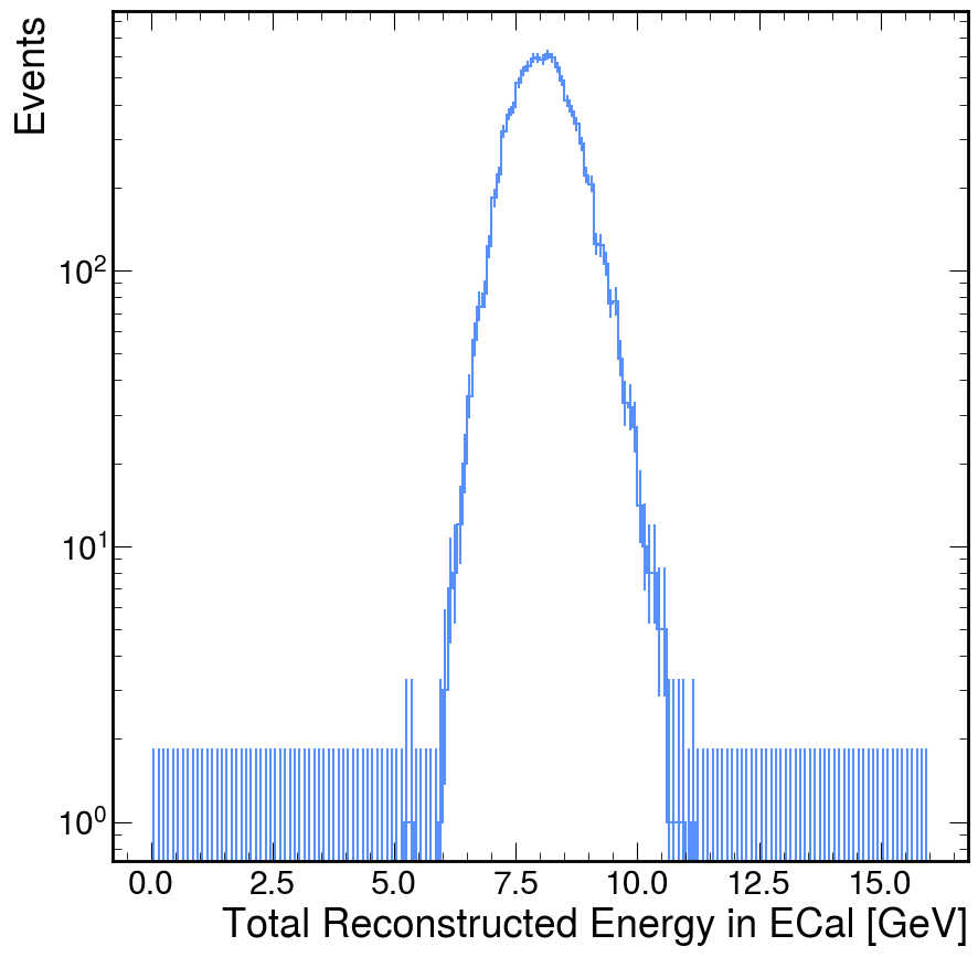
As an example, and to show the power of "vectorization", I am going to calculate the total energy reconstructed within the ECal.
These lines are often short but incredibly dense. Do not be afraid to try a few out and see the results, changing the input axis,
as well as other branches of events. While it can be difficult to find the right expression to do the manipulation you wish,
trying different expressions is an incredibly quick procedure and one that I would enourage you to do. Instead of assigning
the result to a variable, you can even just print it directly to the console like events above so you can see the resulting
shape and a few example values.
awkward's website is growing with documentation and has a detailed reference of the available commands.
Nevertheless, you can find more help on numpy's website whose syntax and vocabulary is a main inspiration for awkward.
Specifically, I would guide folks to What is NumPy and the
NumPy Beginners Guide to be given helpful definitions of the relevant vocabulary
("vectorization", "array", "axis", "attribute" to name a few).
%%time
# add up the energy_ along axis 1, axis 0 is the "outermost" axis which is indexed by event
total_ecal_rec_energy = ak.sum(events['EcalRecHits_test.energy_'], axis=1)
CPU times: user 5.99 ms, sys: 2 ms, total: 7.99 ms
Wall time: 7.34 ms
Fill Histogram
Filling a histogram is where we condense a variable calculated for many events into an object that can be viewed and interpreted.
While numpy and matplotlib have histogram filling
and plotting that work well. The hist package gives
a more flexible definition of histogram, allowing you to define histograms with more axes, do calculations with histograms
(e.g. sum over bins, rebin, slicing, projection), and eventually plot them.
We won't go into multi-dimensional (more than one axis) histograms or histogram calcuations here,
but the links below give a helpful overview of available options.
- hist
- hist indexing (the stuff you can put between square brackets)
%%time
# construct the histogram defining a Regular (Reg) binning
# I found this binning after trying a few options
tere_h = hist.Hist.new.Reg(160,0,16,label='Total Reconstructed Energy in ECal [GeV]').Double()
# fill the histogram with the passed array
# I'm dividing by 1000 here to convert the MeV to GeV
tere_h.fill(total_ecal_rec_energy/1000.)
CPU times: user 1.18 ms, sys: 44 µs, total: 1.23 ms
Wall time: 1.26 ms
Double() Σ=10000.0
Plot Histogram
The final step is converting our histogram into an image that is helpful for us humans! hist connects to the standard matplotlib through a styling package called mplhep. Both of which have documentation sites that are helpful to browse so you can gain an idea of the available functions.
- matplotlib is used extensively inside and outside HEP, I often find an immediate answer with a simple internet search (e.g. searching
plt change aspect ratiotells you how to change the aspect ratio of your plot). - mplhep is a wrapper around matplotlib for HEP to do common things like plot histograms.
tere_h.plot()
plt.yscale('log')
plt.ylabel('Events')
plt.show()
Round-and-Round We Go
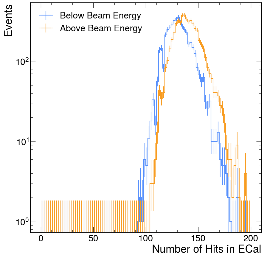
Now, in almost all of my analyses, one plot just immediately opens the door to new questions. For example, I notice that this total energy plot is rather broad, I want to see why that is. One idea is that it is simply a function of how many hits we observed in the ECal. There are many ways to test this hypothesis, but I'm going to do a specific method that showcases a specific tool that is extremely useful: boolean slicing (awkward's implementation is inspired by numpy's boolean slicing but it also interacts with the idea of broadcasting between arrays).
I also showcase a helpful feature of hist where if the first axis is a StrCategory, then
the resulting plot will just overlay the plots along the other axis.
You'll notice that, while I'm manipulating the data, filling a histogram, and plotting the histogram, I do not need to re-load the data. This is by design. Jupyter Lab (and the notebooks it interacts with) use an interactive Python "kernel" to hold variables in memory while you are using them. This is helpful to avoid the time-heavy job of loading data into memory, but it can be an area of confusion. Be careful to not re-use variable names and create new notebooks often!
nhits_by_tere_h = (
    hist.Hist.new
    .StrCategory(['Below Beam Energy','Above Beam Energy'])
    .Reg(100,0,200,label='Number of Hits in ECal')
    .Double()
)
n_ecal_hits = ak.count(events['EcalRecHits_test.id_'], axis=1)
nhits_by_tere_h.fill(
    'Below Beam Energy',
    n_ecal_hits[total_ecal_rec_energy < 8000.]
)
nhits_by_tere_h.fill(
    'Above Beam Energy',
    n_ecal_hits[total_ecal_rec_energy > 8000.]
)
nhits_by_tere_h.plot()
plt.yscale('log')
plt.ylabel('Events')
plt.legend()
plt.show()
Using ldmx-sw Directly
As you may be able to pick up based on my tone, I prefer the (efficient) python analysis
method given before using uproot, awkward, and hist. Nevertheless, there are two
main reasons I've had for putting an analysis into the ldmx-sw C++.
- Longevity: While the python ecosystem evolving quickly is helpful for obtaining new features, it can also cause long-running projects to "break" -- forcing a refactor that is purely due to upstream code changes.1 Writing an analysis into C++, with its more rigid view on backwards compatibility, essentially solidifies it so that it can be run in the same way for a long time into the future.
- Non-Vectorization: In the previous chapter, I made a big deal about how most
analyses can be vectorizable and written in terms of these pre-compiled and fast
functions. That being said, sometimes its difficult to figure out how to write
an analysis in a vectorizable form. Dropping down into the C++ allows analyzers
to write the
forloop themselves which may be necessary for an analysis to be understandable (or even functional).
This longevity issue can be resolved within python by "pinning" package versions so that all developers of the analysis code use the same version of python and the necessary packages. Nevertheless, this "pinning" also prevents analyzers from obtaining new features or bug fixes brought into newer versions of the packages.
The following example is stand-alone in the same sense as the prior chapter's jupyter notebook. It can be run from outside of the ldmx-sw repository; however, this directly contradicts the first reason for writing an analysis like this in the first place. I would recommend that you store your analyzer source code in ldmx-sw or the private ldmx-analysis. These repos also contain CMake infrastructure so you can more easily share code common amongst many processors.
Set Up
I am going to use the same version of ldmx-sw that was used to generate
the input events.root file. This isn't strictly necessary - more often
than not, newer ldmx-sw versions are able to read files from prior ldmx-sw
versions.
This tutorial uses a feature introduced into ldmx-sw in v4.0.1. One can follow the same general workflow with some additional changes to the config script described below.
cd work-area
denv init ldmx/pro:<ldmx-sw-version>
where <ldmx-sw-version> is a version of ldmx-sw that has been released. The version of ldmx-sw you want to use depends on what features
you need and input data files you want to analyze.
The following code block shows the necessary boilerplate for starting
a C++ analyzer running with ldmx-sw.
// filename: MyAnalyzer.cxx
#include "Framework/EventProcessor.h"

#include "Ecal/Event/EcalHit.h"

class MyAnalyzer : public framework::Analyzer {
 public:
  MyAnalyzer(const std::string& name, framework::Process& p)
    : framework::Analyzer(name, p) {}
  ~MyAnalyzer() override = default;
  void onProcessStart() override;
  void analyze(const framework::Event& event) override;
};

void MyAnalyzer::onProcessStart() {
  // this is where we will define the histograms we want to fill
}

void MyAnalyzer::analyze(const framework::Event& event) {
  // this is where we will fill the histograms
}

DECLARE_ANALYZER(MyAnalyzer);
And below is an example python config called ana-cfg.py that I will
use to run this analyzer with fire. It assumes to be in the same
place as the source file so that it knows where the files it needs
are located.
from LDMX.Framework import ldmxcfg
p = ldmxcfg.Process('ana')
p.sequence = [ ldmxcfg.processor_from_file('MyAnalyzer.cxx', needs=['SimCore_Event', 'Ecal_Event']) ]
p.input_files = [ 'events.root' ]
p.histogram_file = 'hist.root'
p.pause()
If you are using ldmx-sw < v4.7.0 (but >= v4.0.1), then the processor_from_file function
was named Analyzer.from_file but otherwise works the same.
Unable to Load Library
Unable to Load Library
If you see an error like the one below, you are probably not linking
your stand-alone processor to its necessary libraries.
The configuration script needs to be updated with needs listing
the ldmx-sw libraries that the stand-alone processor needs to be
linked to.
For example, this tutorial uses the Ecal hits defined in the
Ecal/Event area which means we need to add 'Ecal_Event' to
the needs list.
Example error you could see...
$ denv fire ana-cfg.py
---- LDMXSW: Loading configuration --------
Processor source file /home/tom/code/ldmx/website/src/using/analysis/MyAnalyzer.cxx is newer than its compiled library
 /home/tom/code/ldmx/website/src/using/analysis/libMyAnalyzer.so (or library does not exist), recompiling...
 done compiling /home/tom/code/ldmx/website/src/using/analysis/MyAnalyzer.cxx
 ---- LDMXSW: Configuration load complete  --------
 ---- LDMXSW: Starting event processing --------
 Warning in <TClass::Init>: no dictionary for class pair<int,ldmx::SimParticle> is available
 Warning in <TClass::Init>: no dictionary for class ldmx::SimParticle is available
 Warning in <TClass::Init>: no dictionary for class ldmx::SimTrackerHit is available
 Warning in <TClass::Init>: no dictionary for class ldmx::SimCalorimeterHit is available
 Warning in <TClass::Init>: no dictionary for class ldmx::HgcrocDigiCollection is available
 Warning in <TClass::Init>: no dictionary for class ldmx::EcalHit is available
 Warning in <TClass::Init>: no dictionary for class ldmx::CalorimeterHit is available

 ... proceeds to seg fault on getEnergy ...
A quick test can show that the code is compiling and running (although it will not print out anything or create any files).
$ denv time fire ana-cfg.py
---- LDMXSW: Loading configuration --------
Processor source file /home/tom/code/ldmx/website/ldmx-sw-eg/MyAnalyzer.cxx is newer than its compiled library /home/tom/code/ldmx/website/ldmx-sw-eg/libMyAnalyzer.so (or library does not exist), recompiling...
done compiling /home/tom/code/ldmx/website/ldmx-sw-eg/MyAnalyzer.cxx
---- LDMXSW: Configuration load complete  --------
---- LDMXSW: Starting event processing --------
---- LDMXSW: Event processing complete  --------
7.79user 0.74system 0:08.55elapsed 99%CPU (0avgtext+0avgdata 601516maxresident)k
264inputs+2480outputs (0major+223914minor)pagefaults 0swaps
MyAnalyzer needed to be compiled which increased the time it took to run.
Re-running again without changing the source file allows us to skip this compilation step.
$ denv time fire ana-cfg.py
---- LDMXSW: Loading configuration --------
---- LDMXSW: Configuration load complete  --------
---- LDMXSW: Starting event processing --------
---- LDMXSW: Event processing complete  --------
3.52user 0.14system 0:03.66elapsed 100%CPU (0avgtext+0avgdata 325828maxresident)k
0inputs+0outputs (0major+58137minor)pagefaults 0swaps
Notice that we still took a few seconds to run.
This is because, even though MyAnalyzer isn't doing anything with the data,
fire is still looping through all of the events.
You do not need to include time when running.
I am just using it in this tutorial to give you a sense of how long
different commands run.
Load Data, Manipulate Data, and Fill Histograms
While these steps were separate in the previous workflow, they all share the same process
in this workflow. The data loading is handled by fire and we are expected to write the
code that manipulates the data and fills the histograms.
I'm going to look at the total reconstructed energy in the ECal again. Below is the updated
code file. Notice that, besides the additional #include at the top, all of the changes were
made within the function definitions.
// filename: MyAnalyzer.cxx
#include "Framework/EventProcessor.h"

#include "Ecal/Event/EcalHit.h"

class MyAnalyzer : public framework::Analyzer {
 public:
  MyAnalyzer(const std::string& name, framework::Process& p)
    : framework::Analyzer(name, p) {}
  ~MyAnalyzer() override = default;
  void onProcessStart() override;
  void analyze(const framework::Event& event) override;
};

void MyAnalyzer::onProcessStart() {
  histograms_.create(
      "total_ecal_rec_energy",
      "Total ECal Rec Energy [GeV]", 160, 0.0, 16.0
  );
}

void MyAnalyzer::analyze(const framework::Event& event) {
  const auto& ecal_rec_hits{event.getCollection<ldmx::EcalHit>("EcalRecHits","")};
  double total = 0.0;
  for (const auto& hit : ecal_rec_hits) {
    total += hit.getEnergy();
  }
  histograms_.fill("total_ecal_rec_energy", total/1000.);
}

DECLARE_ANALYZER(MyAnalyzer);
Look at the documentation of the HistogramPool
to see more examples of how to create and fill histograms.
Missing Histograms
Missing Histograms
If the output histogram file you are writing to does not receive any histograms despite
you following the above procedure, you are probably working with an older version of
ldmx-sw. In v4.5.1 ldmx-sw and earlier, you needed to include getHistoDirectory()
at the beginning of your onProcessStart function.
In order to run this code on the data, we need to compile and run the program.
The special processor_from_file function within the config script handles this in
most situations for us.
Below, you'll see that the analyzer is re-compiled into the library while
fire is loading the configuration and then the analyzer is used during event processing.
$ denv fire ana-cfg.py
---- LDMXSW: Loading configuration --------
Processor source file /home/tom/code/ldmx/website/ldmx-sw-eg/MyAnalyzer.cxx is newer than its compiled library /home/tom/code/ldmx/website/ldmx-sw-eg/libMyAnalyzer.so (or library does not exist), recompiling...
done compiling /home/tom/code/ldmx/website/ldmx-sw-eg/MyAnalyzer.cxx
---- LDMXSW: Configuration load complete  --------
---- LDMXSW: Starting event processing --------
---- LDMXSW: Event processing complete  --------
Now there is a new file hist.root in this directory which has the histogram we filled stored within it.
$ denv rootls -l hist.root
TDirectoryFile  Apr 30 22:30 2024 MyAnalyzer "MyAnalyzer"
$ denv rootls -l hist.root:*
TH1F  Apr 30 22:30 2024 MyAnalyzer_total_ecal_rec_energy  ""
In v4.5.2 of ldmx-sw, the histogram pooling was changed to avoid referencing the name of the analyzer in both the directory and the histogram itself. Before this release, the histogram would have been located at "MyAnalyzer/MyAnalyzer_total_ecal_rec_energy" but if you are using this release or newer, the same histogram would be located at "MyAnalyzer/total_ecal_rec_energy".
Plotting Histograms
Viewing the histogram with the filled data is another fork in the road.
I often switch back to the Jupyter Lab approach using uproot to load histograms from hist.root
into hist objects that I can then manipulate and plot with hist and matplotlib.
Accessing Histograms in Jupyter Lab
Accessing Histograms in Jupyter Lab
I usually hold the histogram file handle created by uproot and then use the to_hist() function
once I find the histogram I want to plot in order to pull the histogram into an object I am
familiar with. For example
f = uproot.open('hist.root')
h = f['MyAnalyzer/MyAnalyzer_total_ecal_rec_energy'].to_hist()
h.plot()
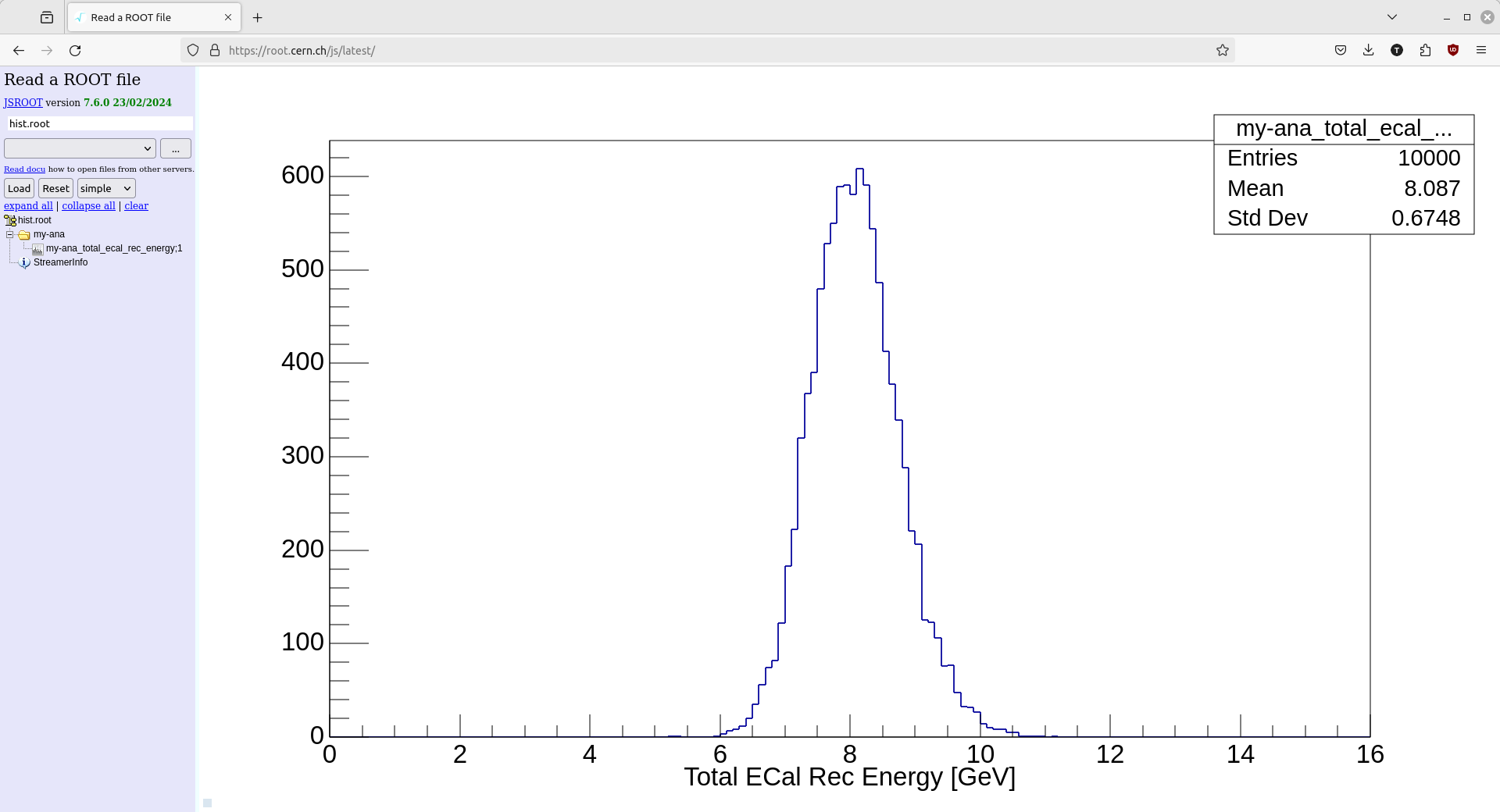
But it is also very common to view these histograms with one of ROOT's browsers.
There is a root browser within the dev images (via denv rootbrowse or ldmx rootbrowse),
but I also like to view the histogram with the online ROOT browser.
Below is a screenshot of my browser window after opening the hist.root file and then
selecting the histogram we filled.
Pre-4.0.1 Standalone Analyzers
PR #1310 goes into detail on the necessary changes, but - in large part - we can mimic the feature introduced in v4.0.1 with some additional python added into the config file.
The file below hasn't been thoroughly tested and may not work out-of-the-box. Please open a PR into this documentation if you find an issue that can be patched generally.
from pathlib import Path

class StandaloneAnalyzer:
    def __init__(self, instance_name, class_name):
        self.instanceName = instance_name
        self.className = class_name
        self.histograms = []

    @classmethod
    def from_file(cls, source_file):
        if not isinstance(source_file, Path):
            source_file = Path(source_file)
        if not source_file.is_file():
            raise ValueError(f'{source_file} is not accessible.')

        src = source_file.resolve()

        # assume class name is name of file (no extension) if not provided
        class_name = src.stem
        instance_name = class_name
        lib = src.parent / f'lib{src.stem}.so'
        if not lib.is_file() or src.stat().st_mtime > lib.stat().st_mtime:
            print(
                f'Processor source file {src} is newer than its compiled library {lib}'
                ' (or library does not exist), recompiling...'
            )
            import subprocess
            # update this path to the location of the ldmx-sw install
            # this is the correct path for production images
            ldmx_sw_install_prefix = '/usr/local'
            # for dev images, you could look at using
            #ldmx_sw_install_prefix = f'{os.environ["LDMX_BASE"]}/ldmx-sw/install'
            subprocess.run([
                'g++', '-fPIC', '-shared', # construct a shared library for dynamic loading
                '-o', str(lib), str(src), # define output file and input source file
                '-lFramework', # link to Framework library (and the event dictionary)
                '-I/usr/local/include/root', # include ROOT's non-system headers
                f'-I{ldmx_sw_install_prefix}/include', # include ldmx-sw headers
                f'-L{ldmx_sw_install_prefix}/lib', # include ldmx-sw libs
            ], check=True)
            print(f'done compiling {src}')

        ldmxcfg.Process.addLibrary(str(lib))
        instance = cls(instance_name, class_name)
        return instance

p = ldmxcfg.Process('ana')
import os
p.sequence = [ StandaloneAnalyzer.from_file('MyAnalysis.cxx') ]
p.inputFiles = [ 'events.root' ]
p.histogramFile = 'hist.root'
Running and Configuring fire
The fire application is used for simulation, reconstruction, and analysis of data from the LDMX experiment. The application receives its configuration for a given purpose by interpreting a python script which contains instructions about what C++ code to run and what parameters to use. The python script is not run for each event, but instead is used to determine the configuration of the C++ code which is run for each event.
Brief summary of running fire
From the commandline, the application is run as follows:
$ denv fire {configuration_script.py} [arguments for configuration script]
The configuration script language is discussed in more detail below.
Other prefixes besides denv
Other prefixes besides denv
denv was pre-dated by a set of bash functions whose root command was ldmx.
This means you can see ldmx as the main prefix for commands that
should be running within the ldmx-sw environment.
In most cases, one can simply replace ldmx with denv since they have
similar design goals.
Developers of ldmx-sw may also be using the recipe manager just and run
the above with just as the prefix. This just (pun intended) runs denv fire
under-the-hood, so it is also equivalent.
Configuration script arguments
Arguments after the .py file on the commandline will be passed to the script as normal arguments to any python script.
These can be used in many ways to adjust the behavior of the script. Some examples are given below in the Tips and Tricks section.
Processing Modes
There are two processing modes that fire can run in which are defined by the presence of input data files1.
If there are no input data files, then fire is in Production Mode while if there are input data files, then
fire is in Reconstruction Mode. The names of these two modes originate from how fire is used in LDMX research.
In this context, an "input data file" is a data file previously produced by fire. There can be other types of data that are "input" into fire but unless fire is actually treating those input files as a reference, fire is considered to be in "Production Mode". See the input_files configuration parameter below.
The Process Object
The Process object represents the overall processing step. It must be included in any fire configuration. When the Process is constructed, the user must provide a processing pass name. This processing pass name is used to identify the products in the data file and cannot be repeated when later processing the same file. The pass name is useful when a file has been processed multiple times -- for example, when reprocessing a file with new calibration constants.
As an example, the pass name is practice, so the line which constructs the Process is:
p = ldmxcfg.Process("practice")
As part of our drive to have better organized Python configuratin modules, we applied common
Python linting and formatting rules to ldmx-sw. This led to many parameters being changed
from camelCase to snake_case marked by the release of v4.6.0 of ldmx-sw.
If you are using a version of ldmx-sw prior to v4.6.0, then you will likely need to change
any snake_case parameter name in this example to camelCase although that is not true
in all cases.
The documentation written here does not necessarily fix this rename in all places. Please contribute if you find a place that needs to be updated!
Here is a list of some of the most important process options and what they control.
It is encouraged to browse the python modules themselves for all the details,
but you can also call help(ldmxcfg.Process) in python to see the documentation.
pass_name(string)- required Given in the constructor, tag for the process as a whole.
- For example:
"10MeVSignal"for a simulation of a 10MeV A'
run(integer)- Unique number identifying the run
- For example:
9001 - Default is
0
max_events(integer)- Maximum number of events to run for
- Required for Production Mode (no input files)
- In Reconstruction Mode, the number of events that are run is the number of events in the input files unless this parameter is positive and less than the input number.
- For example:
9000
output_files(list of strings)- List of files to output events to
- Required to be exactly one for Production Mode, and either exactly one or exactly the number of input files in Reconstruction Mode.
- For example:
[ "output.root" ]
input_files(list of strings)- List of files to read events in from
- Required if no output files are given
- For example:
[ "input.root" ]
histogram_file(string)- Name of file to put histograms and ntuples in
- For example:
"myHistograms.root"
sequence(list of event processors)- Required to be non-empty
- List of processors to run the events through (in the order given)
- For example:
[ mySimulator, ecalDigis, ecalRecon ]
keep(list of strings)- List of drop/keep rules to help ldmx-sw know which collections to put into output file(s)
- Slightly complicated, see the documentation of EventFile
- For example:
[ "drop .*SimHits.*" , "keep Ecal.*" ]
skim_default_is_keep(bool)- Should the process keep events unless told to drop by a processor?
- Default is
True: events will be kept unless processors usesetStorageHint. - Use
skim_default_is_drop()orskim_default_is_save()to modify
skim_rules(list of strings)- List of processors to use to decide whether an event should be stored in the output file (along with the default given above).
- Has a very specific format, use
skim_consider( processorName )to modifyprocessor_nameis the instance name and not the class name
- For example, the Ecal veto chooses whether an event should be kept or not depending on a lot of physics stuff. If you only want the events passing the veto to be saved, you would:
p.skim_default_is_drop() #process should drop events unless specified otherwise
p.skim_consider('ecalVeto') #process should listen to storage hints from ecalVeto
log_frequency(int)- How frequently should the processor tell you what event number it is on?
- Default is
-1which is never.
logger.term_level(int)- how severe messages should be before they are printed to the terminal
- default is
2which is warnings and above, the event number printing is at level1(info)
Configuration File Basics
Often times, the script that is passed to fire to configure how ldmx-sw runs and processes data is called a "config script" or even simply "config". This helps distinguish these python files from other python files who have different purposes (like filling histograms or creating plots).
There are many configs stored within ldmx-sw itself which mostly exist to help developers quickly test any code developments they write. These examples, while often complicated at first look, can be helpful for a new user wishing to learn more about how to write their own config for ldmx-sw.
.github/validation_samples/<name>/config.py: configs used in automatic PR validation tests, these have a variety of simulations as well as the full suite of emulation and reconstruction processors with ldmx-swBiasing/test/: configs used to help manually test developments in the Biasing and Simulation code, these mostly just have simulations and do not contain emulation and reconstruction processorsexampleConfigsdirectory within modules: configs written by module developers to help describe how to use the processors they are developing
In order to help guide your browsing, below I've written two example configs that will not run but they do show code snippets that are similar across a wide variety of configs.
In all configs, there will be the creation of the Process object where the name of that pass is defined and there will be some lines defining the p.sequence of processors
that will be run to process the data.
Additional notes:
- Using the variable name
pfor theProcessobject is just convention and is not strictly necessary; however, it does lend itself nicely to sharing bits of code between configs. - Most of the time, especially for processors that are already written into ldmx-sw, the construction of a processor is put into its own python module so that the C++ class name, the module name, and any other parameters can be properly spelled once and used everywhere.
Minimal Production Config
In Production Mode, there won't be a p.input_files line but there will be a line setting p.run to some value.
from LDMX.Framework import ldmxcfg
p = ldmxcfg.Process('mypass')
p.output_files = ['output_events.root']
p.run = 1
p.sequence = [
  ldmxcfg.make_processor('my_producer','some::cpp::MyProducer','Module')
]
Minimal Reconstruction Config
In Reconstruction Mode, there will be a p.input_files line but since p.run will be ignored it is often omitted.
from LDMX.Framework import ldmxcfg
p = ldmxcfg.Process('myreco')
p.input_files = ['input_events.root']
p.output_files = ['rereco_input_events.root']
p.sequence = [
  ldmxcfg.make_processor('my_reco', 'some::cpp::MyReco', 'Module')
]
Structure of Event Processors
In ldmx-sw, processors have a structure that overlap between C++ and python where we attempt to use the strengths of both languages.
In C++, we do all the heavy lifting and try to utilize the language's speed and efficiency.
In python, we do the complicated task of assigning values for all of the configuration parameters, regardless of type.
C++
The C++ part of the event processor is a derived class that has multiple different methods accessing different parts at different points of time along the processing chain. I am not going to go through all of those parts in detail, but I will focus on two methods that are used in almost all processors.
The configure method of your event processor is given an object called Parameters which contains all the parameters retrieved from python (more on that later).
This method is called immediately after the processor is constructed, so it is the place to set up your processor and make sure it will do what you want it to do.
The produce (for Producers) or analyze (for Analyzers) method of your event processor is given the current event object.
With this event object, you can access all of the objects that have been previously stored into it and (for Producers only)
put new event objects into it.
Here is an outline of a Producer with these two methods. This was not tested. It is just here for illustrative purposes.
// in the header file
// ldmx-sw/MyModule/include/MyModule/MyProducer.h

namespace mymodule {
/**
 * We inherit from the Producer class so that
 * the application can know what to do with us.
 */
class MyProducer : public Producer {
 public:
  /**
   * Constructor
   * Required to match the structure set up by Producer
   */
  MyProducer(const std::string& name, Process& p) : Producer(name, p) {}

  /**
   * Destructor
   * Marked override so that it will be called when MyProducer
   * is destructed via a pointer of type Producer*
   */
  ~MyProducer() override = default;

  /**
   * Configure this instance of MyProducer
   *
   * We get an object storing all of the parameters set in the python.
   */
  void configure(Parameters& params) override;

  /**
   * Produce for the input event
   *
   * Here is where you do all your work on an event-by-event basis.
   */
  void produce(Event& event) override;

 private:
  /// a parameter we will get from python
  int my_parameter_;

  /// another parameter we will get from python
  std::vector<double> my_other_parameter_;
}; // MyProducer
}  // mymodule


// in the source file
// ldmx-sw/MyModule/src/MyModule/MyProducer.cxx

#include "MyModule/MyProducer.h"

namespace mymodule {

void MyProducer::configure(const Parameters& params) {
  my_parameter_ = params.get<int>("my_parameter");
  my_other_parameter_ = params.get<std::vector<double>>("my_other_parameter");

  std::cout << "I also know the name "
      << params.get<std::string>("instance_name")
      << " and class "
      << params.get<std::string>("class_name")
      << " of this copy of MyProcessor" << std::endl;
}

void MyProducer::produce(Event& event) {
  // insert processor's event-by-event work here
}

}  // mymodule

DECLARE_PRODUCER(mymodule::MyProducer);
Python
The python part of the event processor is set up to allow the user to specify the parameters the processor should use. We also define a class in python that will be accessed by the application.
The python class has three objectives:
- Define all of the parameters that the processor requires (and reasonable defaults)
- Include the library that the C++ processor is apart of
- Tell the configuration what the C++ class it links to is
Here is an outline of the python class that would go with the C++ class MyProducer above.
@processor("mymodule::MyProducer", "MyModule")
class MyProducer(Processor) :
    """An outline for a producer configuration in python

    Parameters
    ----------
    my_parameter : int
      An example of an integer parameter
    my_other_parameter : list[float]
      An example of a vector of doubles parameter
    """

    # define the parameters and their defaults
    # the names of the parameters here should match what is in the C++
    my_parameter: int = 5
    my_other_parameter: list[float] = [1.0, 2.0, 3.0]
Now in a configuration script you can create a configuration for MyProducer and (if you want) change some of the parameters to something other than the defaults.
There is a wealth of examples present in ldmx-sw - just look in the python subdirectory of any module - but I want to highlight some specific features that can be helpful.
- writing a
__post_init__function can give you access to the configuration class while it is being constructed so you can do more dynamic things like (for example) having some parameters depend on others (maybe the output name depends on which input is being looked at) - the parameters are spell- and type- checked on the Python side using their spelling and types as written above. This means any parameter changes should be propagated to the
classfirst and then the checker can point out where downstream changes are needed
# in a configuration python script
#   my_producer is the python file in MyModule/python
#   that contains the python class definition of MyProducer
from LDMX.MyModule import my_producer
p.sequence = [
    # the parameters can be set in the constructor
    my_producer.MyProducer(
      instance_name = 'special-name',
      my_parameter = 10 # C++ recieves 10 instead of the default 5
    )
]

# or after creation if something more dynamic is needed
another = my_producer.MyProducer(instance_name = "another")
another.my_parameter = 20
Other Objects
This structure for Event Processors is pretty general, and actually there are other objects in the C++ application that are configured in this way: PrimaryGenerators, UserActions, ConditionsObjectProviders, DarkBremModels, BiasingOperators.
Drop Keep Rules
By default, all data that is added to an event (via event.add within a produce function)
is written to the output data file. This is a helpful default because it allows users to
quickly write a new config and see everything that was produced by it.
Nevertheless, it is often helpful to avoid storing specific event objects within the output file mostly because the output file is getting too large and removing certain objects can save disk space without sacrificing too much usability for physics analyses. For this purpose, our processing framework has a method for configuring which objects should be stored in the output file. This configuration is colloquially called "drop keep rules" since some objects can be "dropped" during processing (generated in memory but not written to the output file) while others can be explicitly kept (i.e. written to the output file).
The drop keep rules are written in the config as a python list of strings
# p is the ldmxcfg.Process object created earlier
p.keep = [ '<rule0>', '<rule1>', ... ]
the implementation of these rules is done in the
framework::EventFile class
specifically the addDrop function handles the deduction of these rules.
Rule Format
Each rule in the list should be a string with a single space.
decision expression
decisionis one of three strings:drop,keep, andignore.expressionis a regular expression that will be compared against the branch names
decision
As the name implies, this first string is the definition of what should happen to an event object that this rule applies to. It must exactly match one of the strings below and must appear at the start of the rule string.
drop: event objects matchingexpressionare readable during processing but not written to the output filekeep: event objects matchingexpressionare written to the output file (the default for all objects)ignore: event objects matchingexpressionare not read from the input file at all and are invisible to processors
drop lets processors still read the collection during processing — it just will not appear in the
output file. ignore goes further: the branch is not registered in the event product list at all,
so processors cannot access it even if they try. Use ignore when you want to completely hide
collections from a previous pass (e.g. intermediate "test" pass data) while reprocessing with a
new pass.
A drop or ignore rule that would match EventHeader will raise an error at startup.
The EventHeader is required by the framework and cannot be removed.
expression
This regular expression has been tested against basic sub-string matching and it is advised to stay within the realm of sub-string matching.
Since we append the pass name of a process to the end of event objects created within that
process, we expect this expression to be focused on matching the prefix of the full branch name.
Thus, if an expression does not end in a * character, one is appended automatically.
Ordering
The rules are applied in order and can override one another. This allows for more complicated decisions to be made. In essence, the last rule in the list whose expression matches the event object's name is the decision that will be applied.
Drop all scoring plane hit collections except the one for the ECal.
p.keep = [
    'drop .*ScoringPlane.*',
    'keep EcalScoringPlane.*'
]
When reprocessing data, you can hide all collections from a previous pass so that processors cannot accidentally read old data. New collections with the current pass name will still be created normally.
p.keep = [
    'ignore test',  # hide all branches with pass name "test"
]
In a very tight disk space environment, you can drop all event objects and then only keep ones you specifically require. In general, this is not recommended.
p.keep = [
    'drop .*',
    'keep HcalHits.*',
    'keep EcalHits.*',
]
The above would produce a file with only the Hcal and Ecal hits. A warning will be printed
at startup when an all-matching drop or ignore rule is detected.
Make sure to thoroughly test your config with p.keep set to confirm that
everything you need is in the output file. It is very easy to mis-type one of these patterns
and prevent anything from being written to the output file.
Event Skimming
Another feature of our event processing framework is selecting out only certain events to be written into the output file. This is colloquially called "skimming" and is helpful for many reasons, primarily for users to be able to not waste disk space on events that are not interesting for an analysis.
Since not writing events into the output file is an inherently destructive feature, event skimming will only operate if both the config and the processors being run by the config support it. Both play a part in how the choice to keep an event is made and so they are described below.
The StorageControl class in the processing framework is what handles the event skimming decisions and the input from the config and processors.
Processor
On the C++ side of things, processors can use their protected member function setStorageHint
to "hint" to the framework what that processor wants to happen to the event. The argument
to this function is a framework::StorageControl::Hint value as well as a string that can
be used to give a more detailed "purpose".
Hints are then used to algorithmically decide if an event should be written to the output file (kept) or not (dropped). Only hints passing the "listening rules" (see below) are included in this algorithm.
Must*: "must"-style hints are dominant. If any processor provides a "must" hint, then that decision is made.MustDroptakes precendence overMustKeepif both are provided.Should*: "should"-style hints are less forceful and are just used to tally votes. A simple majority of should hints is used to make the decision if no must hints are provided.- If there is a tie (including if no hints are provided), then the default decision is made.
Config
The config script can alter which processors the framework will "listen" to when deciding what to do with an event by checking for specific processor names and (optionally) only specific "purpose" strings from that processor. In addition, the config script defines what the default decision is in the case of no hints or a tie in voting.
Listening Rules
The format of the string representing a listening rule is a bit complicated, so it is best
to just use the p.skim_consider function when defining which processors you wish to "listen"
to (or "consider") when making a skimming decision. Most commonly, a user just has one processor
that they want to make the skimming decision and in this case you can just provide the processors
name.
p.skim_consider(my_processor.instanceName)
Technically, the listening rules use regular expressions for both the processor name and the purpose, so one could get quite fancy about which processors (and purposes) are selected. This more intricate skimming method has not been well tested.
Default Decision
The default storage decision is what will be used if no processors that are being listened
to provide a hint during processing. Since the default configuration is to listen to no
processors at all, the default configuration of the default decision is to keep i.e. without
any config changes, we keep all events that are processed. Without changing this,
you could have a processor that explicity "drops" events and update the config to consider
this processor in order to run over events and drop the "uninteresting" ones
(using p.skim_consider like above).
On the other hand, we could set the default decision to drop all the events and instead have a processor specifically "keep" events that are interesting. In this case, you would want to add the following to your config.
p.skim_default_is_drop()
along with a p.skim_consider so that something ends up in your output event file.
This style of event dropping is geared more towards readout, reconstruction, and analysis decisions where the event is already fully created in memory and we just want to make a decision about it.
In the simulation, we also allow for events to be "aborted" in the middle of creating it so that we can end the event early and save computing resources from being wasted on an event we've decided is not interesting (for whatever reason). This style of "dropping" events is more commonly called "filtering" the simulation and is more complicated than what is described here since it operates during the Geant4 simulation.
Tips and Tricks
Command Line Arguments
Command Line Arguments
Python has an easy-to-use argument parsing library. This library can be used within an ldmx-sw configuration script in order to change the parameters you are passing to the processors or even to change which processors you use.
For example, I use the code snippet often to pass inputs to the process.
import argparse
from pathlib import Path

parser = argparse.ArgumentParser()
parser.add_argument('run_number',type=int,help='run number for this simulation run')
parser.add_argument('-o','--out-dir',type=Path,help='output directory to write event data to')
args = parser.parse_args()

from LDMX.Framework import ldmxcfg
p = ldmxcfg.Process('example')
p.run = args.run_number
p.output_file = [
  str(args.out_dir / f'my_special_simulation_run_{p.run:04d}.root')
]

# rest of configuration
Looking at the argparse library linked above is highly recommended since it has a lot of flexibility and can make passing arguments into your config very easy.
Manipulating File Paths
Manipulating File Paths
Python's pathlib library is helpful for doing the common tasks of finding files, listing files, and making a new file path.
For example, if input_dir is a pathlib.Path for an input directory of ROOT files.
p.input_files = [ str(f) for f in input_dir.iterdir() if f.suffix == '.root' ]
We can also use an input file input_file to get an output file name and an output directory output_dir
to place this file in the directory we want.
p.output_files = [ str(output_dir / (input_file.stem + '_with_my_analyzer.root')) ]
Generating Simulation Samples
The generation of simulation samples is done mainly by the Geant4 package with several additions stored in the SimCore module of ldmx-sw. However, you do not need to know the simulation to this level of depth. The Simulator producer in the SimCore module is your messenger to run the simulation. Here, I will go through its basic usage. For more information about all of the available parameters, please see the documentation on Configuring the Simulation.
Basic Usage
Running the simulation is just like any other producer in ldmx-sw. In your python configuration script, it is required that you have the following lines (or equivalent):
from LDMX.SimCore.simulator import Simulator
mySimulator = Simulator(instance_name="mySimulator")
You can write your own detector description in the gdml format (if you want), but ldmx-sw already comes with several versions of the LDMX detector description. These versions are installed with it and can be accessed with some python (+ cmake!) code:
mySimulator.set_detector('ldmx-det-v15')
Okay, mySimulator now is created and has been given a path to an LDMX detector description.
What else is needed? Well, we need at least one more thing. We need to tell the simulation how to start the simulation. In Geant4 speak, this is called a "Primary Generator". In ldmx-sw, we already have several generators defined (more details on Configuring the Simulation), but for this simple example, we will just import a standard generator.
from LDMX.SimCore import generators
mySimulator.generators = [ generators.single_4gev_e_upstream_tagger() ]
Now you can add mySimulator to the process sequence:
# p is a Process created earlier in your py config script
p.sequence = [
  mySimulator
  #other processors?
]
Remember to tell the process how many events to simulate and where to put them:
p.max_events = 10
p.output_files = [ "mySimulatorOutput.root" ]
Run: denv fire myConfig.py
(or some other prefix running fire within the ldmx-sw environment)
Other Available Templates
There are a lot of commonly used aspects of the simulation, so we have incorporated these common "templates" into the python interface for the simulation. This section is focused on listing these available templates and how to access them.
Generators
Access with: from LDMX.SimCore import generators.
This module contains functions that produce each of the generators. You should always use these helper functions because sometimes the underlying naming conventions may change in future developments. More detail about the generators is in the Generators section of Configuring the Simulation.
Biased Simulations
Several simulations with biased processes have been used frequently in the past, so we have written templates for using simulations with reasonably-defined defaults.
Processes in ECal
Access with: from LDMX.Biasing import ecal.
Processes in Target
Access with: from LDMX.Biasing import target.
Both ecal and target modules have three functions that allow you to choose which process is biased in that volume.
| Function | Description |
|---|---|
photo_nuclear(detector,generator) | PN process biased up and filtered for in (ecal or target) |
electro_nuclear(detector,generator) | EN process biased up and filtered for in target |
dark_brem(massAPrime,lheFile,detector,generator) | Sets A' mass to massAPrime (in MeV) and uses the input LHE file as vertices for the dark brem simulation more detail here |
More Advanced Details
As I said earlier, you can definitely see all of the capabilities of Simulator by looking at the parameters that are available in the documentation (linked above). Two parameters that I would like to point out is preInitCommands and postInitCommands. These parameters are given directly to the Geant4 UI as a string, so you can still access Geant4 directly using these commands.
The hope is to remove any need for Geant4-style messengers inside of ldmx-sw, but we also don't want to re-write all of Geant4, so we provide this method for accessing the simulation library directly.
Simple Configuration
Here is a simple configuration file that should generate a sample of 10 events without any biasing or signal and reconstructs the ECal and HCal hits.
#simpleSim.py

# need the configuration python module
from LDMX.Framework import ldmxcfg

# Create the necessary process object (call this pass "sim")
p = ldmxcfg.Process( "sim" )

# Set the unique number that identifies this run
p.run = 9001
# import a template simulator and change some of its parameters
from LDMX.SimCore import generators
from LDMX.SimCore import simulator

mySim = simulator.simulator( "mySim" )
mySim.set_detector( 'ldmx-det-v12' )
mySim.generators = [ generators.single_4gev_e_upstream_tagger() ]
mySim.description = 'I am a basic working example!'

# import chip/geometry conditions
import LDMX.Ecal.ecal_geometry
import LDMX.Ecal.ecal_hardcoded_conditions
import LDMX.Hcal.hcal_geometry
import LDMX.Hcal.hcal_hardcoded_conditions
# import processor templates
import LDMX.Ecal.digi as ecal_digi
import LDMX.Hcal.digi as hcal_digi
# add them to the sequence
p.sequence = [
    mySim,
    ecal_digi.EcalDigiProducer(),
    ecal_digi.EcalRecProducer(),
    hcal_digi.HcalDigiProducer(),
    hcal_digi.HcalRecProducer()
    ]

# During production (simulation), max_events is used as the number
# of events to simulate.
# Other times (like when analyzing a file), max_events is used as
# a cutoff to prevent fire from running over the entire file.
p.max_events = 10

# how frequently should the process print messages to the screen?
p.log_frequency = 1

# I want to see all of the information messages (the default is only warnings and errors)
p.logger.term_Level = 1

# give name of output file
p.output_files = [ "output.root" ]

# print process object to make sure configuration is correct
# at beginning of run and wait for user to press enter to start
p.pause()
Which SimParticles are saved?
Often, one of the first tasks users of ldmx-sw have is to inspect the simulated particles that exist in an output file to learn about what happened within an event. It is then fairly easy to find out that not all of the simulated particles are actually saved into the output file. One could find this out in multiple ways, but commonly, folks find this out through one of two observations.
- The track IDs (the key in the
std::mapthey are stored in) skip numbers pretty regularly. - A SimParticle's "parent" or "daughter" is missing from the particles saved for that event.
In any case, this naturally leads to confusion; hence, this page trying to explain it.
I should emphasize here that we copy a G4Track into our SimParticle.
Geant4 has chosen to use the word "particle" to mean the definition of a
particle and its properties. Individual particles moving through space and
time are "tracks" in Geant4. We undo this switch-a-roo because we have
other things called "tracks". To further add confusion, parts of our geometry
infrastructure refer to "trajectories" which are also the same thing.
First, it is helpful to be aware of the structure of the stored simulated
particle data. We save this data as a std::map<int, ldmx::SimParticle>
where the key of the map is the Geant4 track ID of the particle (a unique
integer within each event) and the value is a
ldmx::SimParticle
that stores data about the particle.
Motivation
Why not store all of the simulated particles?
The answer to this question is pretty simple: it is a waste of space. When a high energy electron hits a huge block of material, it undergoes a process we call "showering" creating hundreds if not thousands of particles as it interacts with the material. Most of these particles created during a shower are not "interesting" for our purposes, so it is helpful to just skip saving them. We do have the ability to store all of the particles in an event if you desire, you can follow the same instructions provided for storing all simulated particles during re-simulation.
Implementation
We get around this phenomena of showering by only saving a select group of particles during normal simulation which satisfy one (or more) of the following.
- The simulated particle is one of the primary particles
- This is determined by the generators the user provides to the simulation.
- The simulated particle is created in a region with
StoreTrajectoriesset totrue- This is set within the GDML of the detector where we define regions. In all of the current detectors, all of the regions will store trajectories except the calorimeters.
- The simulated particle has its
SaveFlagset totrue- This is determined by any extra
UserActions the simulation has attached to it.
- This is determined by any extra
We do not usually have any UserActions which set the SaveFlag to false because
UserActions which are looking for particular simulated particles are usually trying
to get around the bulk "veto" imposed by the simulation throwing away simulated particles
that were created within the calorimeter region (either the ECal or the HCal).
UserActions that focus on looking for particular particles and making sure they are saved
already exist and can be used as examples. These actions (and their example configs) largely
live within the Biasing module of ldmx-sw.
This config uses several user actions to make sure the a hard brem occurs within the target and that high-energy photon undergoes a Photon-Nuclear (PN) interaction within the ECal. Since the PN interaction is very interesting for us and it happens in the ECal, this config also uses the TrackProcessFilter action which makes sure all particles that were created with the PN interaction are saved.
With this config, the sim particles that exist in the output file fall into three categories.
- Starts outside of the ECal or HCal. This includes the primary electron that started the simulation, but also may include other particles that are created as the electron journeys from the beam into the calorimeters including the high energy photon created in the target.
- Products of a PN Interaction. All particles that are created via the PN interaction are saved. Since a PN interaction is required to happen in the ECal, many of these particles will have daughter track IDs that do not exist in the particle map since they were not created via the PN interaction and thus do not pass the filter.
This config (as the name implies) does not use any user actions and is just here to help test the basic running of a simulation.
With this config, the sim particles that exist are all created upstream of the calorimeters. If you were to look at a distribution of all particles and their starting z location, you would see none of them past ~200 mm where the front of the ECal and HCal are. These particles include the primary electron fied by the generator and any particles it produces on its way to the calorimeters.
This particle saving infrastructure is handled by the
simcore::UserTrackInformation
which stores the save flag referenced earlier and the
simcore::g4user::TrackingAction
which applies the defaults described above as well as passes the save decision onto
the class which creates the SimParticle for a G4Track.
Configuring the Simulation
This page details some of the parameters you can use to tune the simulation to behave how you want it to. This page is manually written and is focused on introducing folks to important parameters. Please refer to the Python Configuration Reference for a more complete list of parameters - many of which are documented from the code itself.
General
Like any other Producer, the simulation is configured by passing parameters to it in the python configuration file.
simulation.parameter_name = parameter_value
The parameter keys, types, accessing locations, and descriptions are documented on this page. A minimal working example is displayed on Generating Simulation Samples
| Parameter | Type | Accessed By | Description |
|---|---|---|---|
detector | string | Simulator | Full path to detector gdml description |
description | string | Simulator and RootPersistencyManager | Concise phrase describing this simulation in a human-readable way |
verbosity | int | Simulator | Integer flag describing how verbose to be |
scoring_planes | string | RunManager | Full path to scoring plane gdml description |
pre_init_commands | vector of strings | Simulator | Geant4 commands to run before the run is initialized |
post_init_commands | vector of strings | Simulator | Geant4 commands to run after the run is initialized |
Biasing
Biasing is helpful for efficiently simulating the detector's response to various events. The biasing parameters are given directly to the simulation and are listed below.
In v3.0.0 of ldmx-sw, we transitioned the biasing operators to be configured by their own Python classes.
Those operators are stored in the SimCore.bias_operators module and are attached to the Simulator class similar to generators and actions.
# config script snippet example for biasing
from LDMX.SimCore import bias_operators
# Enable and configure the biasing
sim.biasing_operators = [
    bias_operators.PhotoNuclear('ecal', 450., 2500., only_children_of_primary=True)
]
Dark Brem Process (Signal)
The signal generation is done by enabling the dark bremsstrahlung process in Geant4.
We do this using another Python configuration class DarkBrem in the SimCore.dark_brem module.
A more full description of the Dark Brem process and how these parameters affect its abilities is described [on its own page]({% link docs/Dark-Brem-Signal-Process.md %}).
The most direct way of starting the dark brem process is to simply activate by providing the minimal parameters for it to run.
# config script snipet example for dark brem
from LDMX.SimCore import dark_brem
db_model = dark_brem.G4DarkBreMModel(lhe)
db_model.threshold = 2. #GeV - minimum energy electron needs to have to dark brem
db_model.epsilon   = 0.01 #decrease epsilon from one to help with Geant4 biasing calculations
sim.dark_brem.activate(ap_mass , db_model)
UserActions
Because of the wide variety and flexibility of Geant4's UserActions, we have implemented a way for these various classes to all be passed along with their parameters. This method is extremely similar to how you create Event Processors and give them parameters. The best way to illustrate how to use one is with an example:
# First create the UserAction, configuring its various parameters
from LDMX.Biasing import filters
target_brem_filter = filters.TargetBremFilter(
    recoil_max_p_threshold = 3000.0, # MeV
    brem_min_energy_threshold = 5000.0 # MeV
)
# Then give the UserAction to the simulation so that it knows to use it
simulation.actions.append( target_brem_filter )
No matter the UserAction, the last line above is how you tell the simulation to use it.
| Parameter | Type | Accessed By | Description |
|---|---|---|---|
actions | vector of UserActions | RunManager | UserActions to plug into simulation |
The details of how each UserAction works and what parameters are used are (read: should be) documented within each of those classes. There are a few user actions that do more technical things modifying how the simulation progresses. The majority of user actions are "filters" of some kind which are explained in a bit more detail below.
Filters
These UserActions filter for specific behavior in the simulation. Some of them abort an event if certain criteria aren't met and others make sure tracks matching certain criteria are saved into the output simulation file.
Access with: from LDMX.Biasing import filters
The first type of filter aborts events if certain requirements aren't met.
| Filter | Requirement on Event |
|---|---|
TargetBremFilter() | "hard-enough" brem in the target (hard-enough defined by the parameters) |
NonFiducialFilter() | electron misses the ECal |
EcalProcessFilter() | PN interaction happens in the ECal |
DeepEcalProcessFilter() | PN interaction happens deeper (larger z) in the ECal |
TargetENFilter() | EN interaction happens in the Target |
TargetProcessFilter() | some specific interaction happens in the target |
TargetDarkBremFilter() | dark brem happens in the target |
EcalDarkBremFilter() | dark brem happens in the ECal |
TaggerVetoFilter() | Primary electron doesn't fall below a certain energy before reaching target |
PrimaryToEcalFilter() | make sure primary electron reaches the Ecal with a minimum energy |
MidShowerNuclearBkgdFilter() | a minimum amount of energy goes into EN and PN interactions in the ECal |
MidShowerDiMuonBkgdFilter() | a minimum amount of energy goes into a muon conversion in the ECal |
TaggerHitFilter() | require a certain number of tagger tracker layers to be hit |
The other type of filter looks for tracks (what Geant4 call's individual particles) in Geant4 that match certain conditions and tell Geant4 (and our simulation) to save them in the output SimParticles collection.
| Filter | Keeps all tracks... |
|---|---|
TrackProcessFilter | produced by a specific interaction (e.g. PN, EN, or dark brem) |
DecayChildrenKeeper | which are children of a specific particle's decay |
Generators
There are a few general options that determine how primaries are generated. These parameters must be passed directly to the simulation (like the biasing parameters).
| Parameter | Type | Accessed By | Description |
|---|---|---|---|
generators | vector of PrimaryGenerators | PrimaryGeneratorManager | List the primary generators to use in this simulation run |
Like UserActions, PrimaryGenerator is a python class that you can create using the LDMX.SimCore.simcfg python module. And actually, there are several helpful functions defined in the LDMX.SimCore.generators python module. These helpful functions return the correct python class and set some helpful defaults. Look at that file for more details. The most widely used primary generator is a simple one: a single 4GeV electron fired from upstream of the tagger. You could use that generator in your simulation with the following lines:
from LDMX.SimCore import generators
simulation.generators = [ generators.single_4gev_e_upstream_tagger() ]
Several of these generators can be used at once, although not all combinations have been tested.
All of these generators have a beam_spot_smear parameter that defines how to smear the primary vertex it generates in each of the Cartesian directions (x,y,z).
A more detailed description of the parameters you can pass the various generators are listed below. All of the python code below requires the LDMX.SimCore.generators module to be imported:
from LDMX.SimCore import generators
Simple Particle Gun
This generator is the basic Geant4 particle gun. It can shoot one particle of a definite position and momentum into the simulation. Create a ParticleGun with:
myParticleGun = generators.Gun( "myParticleGun" )
# set the parameters, for example, to use electrons:
myParticleGun.particle = 'e-'
| Parameter | Type | Accessed By | Description |
|---|---|---|---|
particle | string | ParticleGun | Geant4 name of particle to use |
energy | double | ParticleGun | Energy of primary particle (GeV) |
position | vector of doubles | ParticleGun | Location to shoot particle from (mm) |
time | double | ParticleGun | Time at which to shoot particle (ns) |
direction | vector of doubles | ParticleGun | Direction to shoot particle (unit-less) |
LHE vertices as primaries
This generator copies the primary vertex from an LHE file into our simulation framework. Create one with:
myLHE = generators.Lhe("path/to/file.lhe")
Geant4's General Particle Source
This generator is the "General Particle Source". It is implemented in Geant4, and has too many parameters to copy over into our framework. This means you will pass the GPS commands as strings that will be given to Geant4. Create one with:
myGPS = generators.Gps(
  init_commands = [
    # list of init commands for GPS messenger
  ]
)
| Parameter | Type | Accessed By | Description |
|---|---|---|---|
init_commands | vector of strings | GeneralParticleSource | List of Geant4 commands to configure the General Particle Source |
Multiple Particle Gun
This generator can generate multiple copies of the same primary particle with the same kinematics. The number of primaries it generates can also be Poisson distributed. Create one with:
myMPG = generators.Multi(
  # set the parameters
)
Here are the parameters you have access to:
| Parameter | Type | AccessedBy | Description |
|---|---|---|---|
n_particles | int | MultiParticleGunPrimaryGenerator | number of particles to create (or the mean of the Poisson distribution) |
enable_poisson | bool | MultiParticleGunPrimaryGenerator | Should the number of particles be Poisson distributed? |
pdg_id | int | MultiParticleGunPrimaryGenerator | PDG ID of the particle(s) to be the primary |
vertex | vector of doubles | MultiParticleGunPrimaryGenerator | location of primary vertex to shoot the particle(s) from (mm) |
momentum | vector of doubles | MultiParticleGunPrimaryGenerator | 3-momentum of primary particle(s) (MeV) |
Photonuclear model
The hadronic interaction used by Geant4 in ldmx-sw to perform photonuclear interactions can be configured to load an arbitrary other model from a dynamic library. There are a couple available within ldmx-sw that are listed here but you can add new ones from any library and load them the same way. For details about this, see Alternative photo-nuclear models.
By default, the simulation will be configured to use the default version of the Bertini model that comes with LDMX's version of Geant4. If you want to change to a different model, you can do so through
from LDMX.SimCore import photonuclear_models as pns
simulation.photonuclear_model = pns.SomeModel()
Note that some of these models should probably be used together with a
corresponding filter from Biasing.particle_filter.
| Model | Corresponding filter | Description |
|---|---|---|
BertiniModel | None | Default |
BertiniNothingHardModel | PhotoNuclearTopologyFilter.NothingHardFilter() | A model that forces high energy PN interactions with heavy nuclei to produce events where no product has more than some threshold kinetic energy |
BertiniSingleNeutronModel | PhotoNuclearTopologyFilter.SingleNeutronFilter() | Similar, but requires exactly one neutron with kinetic energy above the threshold. By default, is applied to interactions with any nucleus. |
BertiniAtLeastNProductsModel | A matching version ofPhotoNuclearProductsFilter | Similar, but requires at least N particles of a list of particle IDs (e.g. kaons) in the final state. |
NoPhotoNuclearModel | Removes photonuclear interactions entirely from the simulation |
Re-Simulation
Oftentimes it is helpful to select specific events from a sample and re-run the full simulation of them while storing more simulation detail about what transpired. Thanks to the excellent work by Einar Elén in SimCore #95 we are able to re-run the simulation using an input file and optionally specifying specific events to re-simulate.
In order to properly re-simulate an event, we need to have properly saved the state of the random number generator at the beginning of the event. This is only done for ldmx-sw versions after v3.3.0 so this re-simulation will only function propertly on samples that were generated with a version of ldmx-sw v3.3.0 or newer.
Additionally, the event will only be re-simulated if the same simulation configuration is used, meaning you should find the config script that was originally used to generate the sample before attempting to re-simulate.
Basics
A key component of re-simulation is to keep the physics configuration of the simulation identical to what it was originally. With this in mind, the suggested procedure is to make a copy of the original file used to run the simulation and then make the following changes.
- Use the previous output file as the input file
- Tell the simulator to
resimulatewhen adding it to thep.sequence
For change (1), I usually provide the previous output file as a command
line argument to the fire config script and so I have something like
this in my re-sim config.
import sys
import os
p.inputFiles = [ sys.argv[1] ]
p.outputFiles = [ 'resim_'+os.path.basename(sys.argv[1]) ]
This writes the resim events into a file with the same name as the original
but with a resim_ prefix added into the current directory.
For change (2), this is where you can optionally provide which events you wish to select for re-simulation.
p.sequence = [
  # sim is the simulator object created and configured earlier
  sim.resimulate(which_events = [42])
  # potentially other processors like normal
]
The which_events aregument is a integer list giving the event numbers
from that file that you wish to re-simulate. If which_events is not
given, then all of the events in the input file are re-simulated.
That's it! Running the updated copy of the simulation config will re-simulate events from the original simulation in an identical manner. This plain re-simulation may not be very helpful on its own, so below we have a few other modifications that could be made to make the re-simulation more helpful.
Running additional processors after re-simulation
After running the re-simulation, the output file will contain both the original sim-hit collection from the input file and the new one from the re-simulation. This means that if you want to run any processors after the simulation that use the collections, you either need to manually specify the re-sim pass name or drop the original collection (recommended).
If you want to run producers after the re-simulation, it is usually easiest to do so with a separate configuration that uses the re-simulation output as an input-file and dropping the original collections during the re-simulation.
As an example, if you wanted to run the Ecal reconstruction chain on a resimulation with pass-name "resim"
# Resim config file
p = ldmxcfg.Process('resim')
# ...
p.input_files = ['original_simulation.root'] # Pass name "sim"
p.output_files = ['resimulation.root'] # Pass name "resim"
# Drop all collections that end with SimHits_sim
p.keep ["drop .SimHits_sim"]
And later in your reconstruction config
# Resim config file
p = ldmxcfg.Process('reconstruct')
# ...
p.input_files = ['resimulation.root'] # Pass name "resim"
p.sequence = [
  ecal_digi,
  ecal_reco
]
Alternatively, you can do it all in one configuration but you will have to manually specify the pass name for each processor that relies on simulated hits that you want to use. Unfortunately, different processors have different naming conventions for the pass name parameter so you will have to check manually how to do it for the processor that you are interested in.
# Resim config file
p = ldmxcfg.Process('resim')
# ...
p.input_files = ['original_simulation.root'] # Pass name "sim"
p.output_files = ['resimulation.root'] # Pass name "resim"

# Digi producer needs the raw simhits
ecal_digi = ...
ecal_digi.input_pass_name = 'resim' # Pick the resim version

p.sequence = [
  resim,
  ecal_digi,
  ecal_reco # Doesn't directly rely on simhits, so doesn't need pass name to be specified!
]
The latter approach gets cumbersome if you want to use more than a couple of processors.
Producing more details about specific events
A common use-case for resimulation is when you have a subset of your events that you are particularly interested in (e.g. EcalPN reactions that pass the BDT veto). Repeating the simulation of just those events can allow you to record details that would otherwise consume too much space or insert additional instrumentation into the simulation (either directly in code or with tools/flags from ldmx-sw).
Printing particle histories
In the Biasing submodule, there is a UserAction available that will print out
the full step history for one or more particles in an event. For anything longer
than a couple events, this would entirely swamp the log with excessive detail.
However, if you run the resimulation which only repeats the events you are
interested in, this becomes a powerful tool for understanding what happened
during the simulation.
# Import the utility set of actions from the Biasing submodule
from LDMX.Biasing import util
resim.actions.extend([
  util.StepPrinter(track_id=1), # Print the primary particle
  util.StepPrinter(process_type='photonNuclear'), # Print any photonuclear products
])
Storing all Simulated Particles
The shower that happens in the calorimeters often creates many hundreds or even thousands
of simulated particles. Thus we cannot save all of the simulated particles for all of our
events - otherwise we would run out of storage space on our computers! Checkout
Which SimParticles are saved? to learn more about how this choice
is made. For our purposes here, if your simulation configuration has no UserActions setting
the SaveFlag to false (which is highly likely), then we can insure that the simulation
saves all of the simulated particles by setting StoreTrajectories to true everywhere.
First, make a local copy of the detector you are simulating so that you can reference it within the config script.
cp path/to/ldmx-sw/install/data/detectors/<detector-name>/detector.gdml .
Update this detector to have all StoreTrajectories flags set to true.
sed -i '/StoreTrajectories/ s/false/true/g' detector.gdml
Finally, update the re-simulation config to use this slightly modified detector instead of the original copy at the install location.
# above we construct the simulator object sim
sim.set_detector( '<detector-name>' )
# update the path to use the new root detector.gdml with updated flags
#   here, we use a relative path and so we must run the config from the
#   directory where the edited detector.gdml is
sim.detector = 'detector.gdml'
Now when the re-simulation is run, all of the simulated particles will be in the output file giving you as much detail about the particles and the processes that they underwent as we can give from ldmx-sw (without modifying the C++ source code).
As mentioned earlier, this stores a lot of particles (most of which are not important),
so this should only be done on small numbers of events (less than 100) to avoid the
files from getting too large and unweildy. In a production scenario, it would be better
to write your own UserAction which finds the particles that interest you rather than
storing all of the particles that are created.
No Merging of Ecal Simulated Hits
Similar to the simulated particles, the number of simulated hits in the ECal is generally too large and so we do a somewhat complicated procedure of merging them in order to reduce the size of the output data file. There is a standing issue focused on improving this merging algorithm Issue #1317 and if that issue is resolved, the parameters of the merging will likely change.
The EcalSD class is what handles each of the simulated hits created while Geant4 is
processing an event. It has two parameters for modifying how these hits should be
created.
enable_hit_contribs, ifTrue, allowsEcalSDto createSimCalorimeterHit"contribs" when more than one hit occurs within the same Ecal cell. IfFalse, all hits within a cell are combined by summing their respective energy deposits and choosing the earliest time.- The default is
True.
- The default is
compress_hit_contribsis only used isenable_hit_contribsisTrue. Ifcompress_hit_contribsisTrue, then a new contrib is only created for unique simulated particles. In other words, a contrib for a specific simulated particle is updated with more energy deposited and another deposit time if another hit is made by that simulated particle in the same ECal cell. IfFalse, a new contrib is created for all simulated hits regardless on if any of the contribs originate from the same simulated particle.
The compress_hit_contribs is the parameter which causes the most confusion when interpreting ECal
simulated hit information and so removing it will give you a contrib for each simulated hit created
by Geant4 within the ECal. The code to put into your re-sim config is below.
# sim is a simulator object created earlier
# must be done _after_ sim.setDetector is called
for sd in sim.sensitive_detectors:
    if 'EcalSD' in sd.class_name:
        sd.compress_hit_contribs = False
The ECal digi-emulation and reconstruction pipeline has only been developed and tested with the default settings of the simulated hit merging. This means you should probably remove the ECal pipeline (or prepare yourself to help develop it) if you start playing with these parameters.
Other Detector Designs
The two prior examples are all about storing more information during the re-simulation process
so that certain "special" events can be studied in more detail. One could also imagine studying how
a select set of "special" events behave within a modified detector. Technically, this is easy -
simply change the name provided to set_detector or specify a relative path like is done when
saving all of the sim particles above. However, there is a big caveat.
The random number generation in Geant4 is sequential. This means psuedo-random numbers are "created"
one-after-another and then given to the process requesting a random number. The simulated events will
only be identical if the requests from different functions are done in the same exact order in order
to preserve the assignment of psuedo-random numbers to their roles in the simulation. We can initiate
this process correctly by setting up the RNG (random number generator) to be in the same state as it
was at the beginning of the original simulated event (what we call the eventSeed in the event header
represents this state); however, if the simulation is not configured the same as before, the order of
random number requests can change leading to different simulation results even though we used the same
initial state of the RNG.
With this disucssion of RNGs aside, I can get to the point: The "special-ness" of an event needs to be "decided earlier" than where the detector is being changed. By "special-ness", I mean what happens within the simulation that causes this event to be interesting (for example, a particularly nasty photon-nuclear interaction followed by a kaon decay). By "decided earlier", I mean that this "special-ness" process needs to happen in a detector volume that is processed by Geant4 before any of the detector volumes that are being changed. For example, if we want to inspect how changes to the HCal can help veto particularly nasty ECal photon-nuclear events, that is ok because we are not changing the ECal where the "special" stuff occurs. We cannot change the ECal itself and expect the re-simulation to re-play the same "special" process since the RNG may not follow the same path. Similarly, we cannot change the tagger or recoil or anything upstream of the ECal for fear of it affecting the RNG.
Alternative Photon-Nuclear Models
This page details the options in LDMX-sw that allow you to change the default model used in Geant4 for modelling photo nuclear interactions.
Example use cases:
- Replacing PN products with known complicated PN topologies for comparing different detector geometries
- Replacing the Bertini with other hadronic models
- Instrumenting a model to extend it in some way, e.g. to run the event generator until you produce an event topology that you are interested in, but could in principle be used to do anything you need (e.g. debugging)
A photonuclear model in ldmx-sw is a class that provides Geant4 with an appropriate hadronic interaction to use for \(\gamma A\) interactions. With the standard LDMX version of Geant4, the hadronic model is a modified version of The Bertini Cascade (for details, see sec D and appendix A of arxiv:1808.04219v1).
To load a different model than the default, you change the photonuclear_model parameter of your simulation processor. A couple such models are bundled with ldmx-sw and adding new ones either within or from outside ldmx-sw is a relatively straigh-forward task.
Models generating rare but challenging final states
With all of these models, when a photonuclear interaction occurs the model will rerun the interaction until a particular condition is met for the final state particles. If it took \(N\) attempts to produce that final state, the weight of the event will be multiplied with \(\frac{1}{N}\). You can access the event weight with the event header. This can produce much faster simulations (>10x faster) than a full simulation + skim would do. However, you may need to be careful so that you don't introduce any significant bias to your results. Consider producing a smaller sample first with a regular simulation and comparing it to a sample of the same size made with one of these models. See the Validation module for a good starting point for such comparisons.
Events with one hard neutron
This model will rerun the event generator until we get an event where one neutron is the only particle with kinetic energy above some threshold. By default, this model is applied for interactions with any nucleus and for photons with at least 2.5 GeV of energy. With these settings and a configuration like the standard ECal PN simulation, you could in principle skip the filter but unless you have e.g. a performance reason to do so consider keeping it.
# Assuming your simulator is called mySim
from LDMX.SimCore import photonuclear_models as pn
from LDMX.Biasing import particle_filter


myModel = pn.BertiniSingleNeutronModel()
# These are the default values of the parameters
myModel.hard_particle_threshold=200. # Count particles with >= 200 MeV as "hard"
myModel.zmin = 0 # Apply the model for any nucleus
myModel.emin = 2500. # Apply the model for photonuclear reactions with > 2500 MeV photons
myModel.count_light_ions=True # Don't disregard deutrons, tritons, 3He, or 4He ions when counting hard particles

# Change the default model to the single neutron model
mySim.photonuclear_model = myModel


myFilter = particle_filter.PhotoNuclearTopologyFilter.SingleNeutronFilter()
# Default values
myFilter.hard_particle_threshold = 200. # MeV, use the same as for the model
myFilter.count_light_ions = True # As above

# Add the filter at the end of the current list of user actions.
mySim.actions.extend([myFilter])
Events with no particles with high kinetic energy
This model is very similar to the previous one with one big exception, it is only applied for interactions with tungsten (the zmin parameter is set to 74). Since the ECal consists of more material than just tungsten, this means that some ECal PN-events will not produce the desired final state. If you don't combine the model with a particle filter, you will have ~50% of your events being regular photonuclear reactions. The reason for this cut on the proton number of the target nucleus is that nothing hard events, which generally include very high product multiplicity, are extremely rare for nuclei with few nucleons. These interactions would therefore receive an extremely small event weight or even get stuck repeating the event generation infinitely for e.g. hydrogen.
from LDMX.SimCore import photonuclear_models as pn
from LDMX.Biasing import particle_filter


myModel = pn.BertiniNothingHardModel()
# These are the default values of the parameters
myModel.hard_particle_threshold=200. # Count particles with >= 200 MeV as "hard"
myModel.zmin = 74 # Apply the model tungsten only
myModel.emin = 2500. # Apply the model for photonuclear reactions with > 2500 MeV photons
myModel.count_light_ions=True # Don't disregard deutrons, tritons, 3He, or 4He ions when counting hard particles

# Change the default model to the nothing hard model
mySim.photonuclear_model = myModel

myFilter = particle_filter.PhotoNuclearTopologyFilter.NothingHardFilter()
# Default values
myFilter.hard_particle_threshold = 200. # MeV, use the same as for the model
myFilter.count_light_ions = True # As above

# Add the filter at the end of the current list of user actions.
mySim.actions.extend([myFilter])
Events with hard kaons (or similar particle selections)
The last of the default models in ldmx-sw works similar to the other two but rather than requiring an exact number of hard particles, it requires at least N hard particles of any of a set of particles that you are interested in. The setup comes with a preconfigured version that requries at least one hard kaon in the final state.
from LDMX.SimCore import photonuclear_models as pn
from LDMX.Biasing import particle_filter


myModel = pn.BertiniAtLeastNProductsModel.kaon()
# These are the default values of the parameters
myModel.hard_particle_threshold=200. # Count particles with >= 200 MeV as "hard"
myModel.zmin = 0 # Apply the model to any nucleus
myModel.emin = 2500. # Apply the model for photonuclear reactions with > 2500 MeV photons
myModel.pdg_ids = [130, 310, 311, 321, -321] # PDG ids for K^0_L, K^0_S, K^0, K^+, and K^- respectively
myModel.min_products = 1 # Require at least 1 hard particle from the list above


# Change the default model to the kaon producing model
mySim.photonuclear_model = myModel

myFilter = particle_filter.PhotoNuclearProductsFilter.kaon()

# Add the filter at the end of the current list of user actions.
mySim.actions.extend([myFilter])
Special models
Default Bertini cascade
The default model used is the BertiniModel. Unlike the other models, it does not create any new hadronic process. Rather, it overrides the function responsible from removing the original Bertini cascade process with an empty function.
from LDMX.SimCore import photonuclear_models as pn
# This is the default model
myModel = pn.BertiniModel()
mySim.photonuclear_model = myModel
Disabling photonuclear interactions
The NoPhotoNuclearModel removes the photonNuclear process entirely, preventing Geant4 from performing any photo nuclear reactions. Can be useful for studies where you want to only look at electromagnetic showers with high statistics. Like BertiniModel, it does not create any hadronic process and features an empty ConstructGammaProcess. Note that when using this model, you have to be careful not to use any features of ldmx-sw that require a process with the name photonNuclear to be present. An example of this is the photonuclear bias operators but there may be others.
from LDMX.SimCore import photonuclear_models as pn
myModel = pn.NoPhotoNuclearModel()
mySim.photonuclear_model = myModel
Details
Adding a new model
To add a new model within a library, you need to add a class that inherits from SimCore/PhotoNuclearModel and registering it with the DECLARE_PHOTONUCLEAR_MODEL macro at the end of your source file. This base class has one pure virtual function that you have to implement called ConstructGammaProcess(G4ProcessManager*) with some other virtual functions you can override if you need some behaviour other than the defaults. If you are adding a photonuclear model from outside of SimCore, you need to register SimCore::PhotoNuclearModels as a dependency when setting up your library.
setup_library(module ModuleName
    dependencies
    # Any other dependencies your module has
    SimCore::PhotoNuclearModels
    sources
    # Your source files
)
Finally, you'll need to add a new model to your python configuration and register it as the as the photonuclear model of your simulation processor.
from LDMX.SimCore import photo_nuclear_model, PhotoNuclearModel

@photo_nuclear_model("ClassName", "ModuleName")
class MyModel(PhotoNuclearModel):
    """
       Documentation
    """
    # declare parameters here like a processor


mySim.photonuclear_model = MyModel()
where 'ClassName' matches the namespace and type name that you registered with DECLARE_PHOTONUCLEAR_MODEL and 'ModuleName' is the name of your module (same as you used in the CMake configuration).
ConstructGammaProcess
This is the only member function of simcore::PhotoNuclearModel you have to implement yourself.
It takes a G4ProcessManager that you use to register new processes with Geant4. This function is responsible for creating a G4HadronInelasticProcess with the name "photonNuclear" (the name matters since other parts of ldmx-sw relies on this being the name of the PN process). The process needs to have one G4HadronicInteraction registered with valid energy range and a cross section dataset. For the latter, there is a default implementation you can use in the PhotoNuclearModel class called addPNCrossSectionData(G4HadronInelasticProcess*) const;
A typical implementation would look like the following
namespace mynamespace {
void MyModel::ConstructGammaProcess(G4ProcessManager* processManager) {
    auto photoNuclearProcess{new G4HadronInelasticProcess("photonNuclear", G4Gamma::Definition())};
    auto myInteraction {new MyHadronicInteraction{ // any parameters
    }};
    myInteraction->SetMaxEnergy(15*CLHEP::GeV);
    addPNCrossSectionData(photoNuclearProcess); // If you forget this line, the simulation won't run.
    photoNuclearProcess->RegisterMe(myInteraction);
    processManager->AddDiscreteProcess(photoNuclearProcess);
} // namespace mynamespace
}
DECLARE_PHOTONUCLEAR_MODEL(mynamespace::MyModel);
You can see how the model is used in GammaPhysics.cxx in SimCore but in short the order of operations is the following
- Create an object derived from
PhotoNuclearModeldynamically depending on the python configuration - Call
removeExistingModelto remove the default hadronic process - Call
ConstructGammaProcessto build thephotonNuclearprocess - Set the
photonNuclearprocess to be first in the list of processes for photons. Necessary for the bias operator to work. - Add the \(\gamma \rightarrow \mu\mu\) process
Instrumenting the photonuclear model
Being able to access and query the internals of the photonuclear process can be a powerful tool for understanding what is going on in your simulation. One way to do this is to derive from the hadronic interaction you are intersted in, most likely the bertini cascade (which you find as G4CascadeInterface in Geant4) and override the G4HadFinalState* ApplyYourself(const G4HadProjectile&, G4Nucleus&) function. You can access the event generator version by invoking G4CascadeInterface::ApplyYourself explicitly. This will populate the theParticleChange member variable which is of type G4HadFinalState, and return a pointer to it so the return value from this function can either be the address of theParticleChange or just the pointer directly.
Say you want to know the rate that photonuclear interactions occur with different nuclei, a quick and dirty tool to get an estimate would be to produce a model that tallies the proton number of the target nucleus before running the event generator. The C++ pseudo-code could look like the following
#include <iostream>
#include <vector>

#include "G4CascadeInterface.hh"
#include "G4HadFinalState.hh"
#include "G4HadProjectile.hh"
#include "G4HadronInelasticProcess.hh"
#include "G4HadronicInteraction.hh"
#include "G4Nucleus.hh"
#include "G4ProcessManager.hh"
#include "SimCore/PhotoNuclearModel.h"
namespace simcore {
// Note: G4CascadeInterface is the name of the bertini cascade hadronic interaction in Geant4
class NuclearTally : public G4CascadeInterface {
 public:
  G4HadFinalState* ApplyYourself(const G4HadProjectile& projectile,
                                 G4Nucleus& target) override {
    const int Z{target.GetZ_asInt()};
    nuclear_tally[Z - 1]++;
    return G4CascadeInterface::ApplyYourself(projectile, target);
  }

  NuclearTally() : nuclear_tally(100, 0) {}
  virtual ~NuclearTally() {
    std::cout << "Final tally results" << std::endl;
    int total{0};
    for (int i{0}; i < nuclear_tally.size(); ++i) {
      const auto value{nuclear_tally[i]};
      total += value;
      if (value != 0) {
        std::cout << "Z: " << i + 1 << " -> " << value << std::endl;
      }
    }
    std::cout << "Total: " << total << std::endl;
  }

  std::vector<int> nuclear_tally{};
};

class NuclearTallyModel : public PhotoNuclearModel {
 public:
  NuclearTallyModel(const std::string& name,
                    const framework::config::Parameters& parameters)
      : PhotoNuclearModel{name, parameters} {}
  void ConstructGammaProcess(G4ProcessManager* processManager) override {
    auto photoNuclearProcess{
        new G4HadronInelasticProcess("photonNuclear", G4Gamma::Definition())};
    auto model{new NuclearTally()};
    model->SetMaxEnergy(15 * CLHEP::GeV);
    addPNCrossSectionData(photoNuclearProcess);
    photoNuclearProcess->RegisterMe(model);
    processManager->AddDiscreteProcess(photoNuclearProcess);
  }
};
}  // namespace simcore
DECLARE_PHOTONUCLEAR_MODEL(simcore::NuclearTallyModel);
With a corresponding python object
# the ModuleName is omitted since we are assuming it has been built
# into the default module: SimCore_PhotoNuclearModels
@photo_nuclear_model("simcore::NuclearTallyModel")
class NuclearTally(PhotoNuclearModel):
    pass
Models forcing particular final states
One use case for customizing the process used for photonuclear reaction is to study particular rare final states like single hard neutron events without having to generate a complete simulation set or as an alternative to biasing schemes like the kaon enhancement setup. There is a abstract base class, BertiniEventTopologyProcess, available that makes implementing such models relatively straight-forward with the Bertini cascade. It handles all of the things underneath the hood like cleaning up the memory from unused secondaries automatically.
The process will run the Bertini cascade over and over until some condition is met for the final state. Once an attempt has been succesful, the event weight is incremented based on the number of attempts made. In the example with MyModel above, you would have a G4HadronicInteraction that is derived from BertiniEventTopologyProcess as myInteraction. Typically you want to combine this kind of process with a corresponding filter.
Included models in LDMX-sw
LDMX-sw comes with a couple of these models included that both cover important final states and illustrate how to extend it with new ones.
BertiniNothingHardModel- Runs the event generator until we find an event where no individual particle has more than some threshold energy.
- By default only applied for nuclei with
Z >= 74since these events are much less likely to occur for lighter nuclei. - By default, light ions with kinetic energy above the threshold are counted so that e.g. an event with a 1 GeV deutron isn't considered "Nothing hard".
- Should be paired with a product filter from
LDMX.Biasing.
from LDMX.SimCore import photonuclear_models as pn
model = pn.BertiniNothingHardModel()
model.hard_particle_threshold = 500. # MeV, Default is 200.
model.zmin = 29 # Include Copper, Default is 74 (W)
model.count_light_ions = False # Default is to include
from LDMX.Biasing import particle_filter
mySim.actions.extend([
    particle_filter.PhotoNuclearTopologyFilter().NothingHard()
])
mySim.photonuclear_model = model
BertiniSingleNeutronModel- Similar to the nothing hard model but requires exactly one particle with kinetic energy above the threshold and that the particle in question is a neutron.
- Default applied for any nucleus
- Has a similar corresponding filter in
LDMX.Biasing.PhotoNuclearTopologyFilter
BertiniAtLeastNProductsModel- Takes a list of PDG particle-ids, an energy threshold, and a particle count and requires that at there are at least N particles with ids matching that in the list with kinetic energy above the threshold
- A version suitable for producing events with at least one kaon in the final state can be obtained from
BertiniAtLeastNProductsModel.kaon() - Should be used together with a corresponding filter such as
LDMX.Biasing.PhotoNuclearProductsFilter
Adding your own model for other final states than those that are included with LDMX-sw
An implementation needs to override three functions, acceptProjectile, acceptTarget, and acceptEvent. The first two allow you to define what types of photons and target nuclei you are interested in. If either acceptProjectile or acceptTarget return false, the event generator will only be called once. The choice of what target nuclei to apply the model to requires some care. Since different final states are more or less likely depending on what nucleus the photon interacts with, you can end up producing events with very low event weight or even get stuck trying to repeat the event generation for a final state that is impossible (e.g. producing a single hard neutron from a photonuclear reaction with hydrogen). On the other hand, if you limit your reactions to only occur for tungsten you might be biasing the kinds of final states that are possible to study. To build an understanding for these kinds of issues, you can add a model that does the corresponding bookkeeping for you. For example, if you keep a count of what the target nucleus is for an ECal PN sample, you would find that ~50% of all PN interactions are with other nuclei than tungsten in the v14 detector.
Once you are sure that you are accepting the right kinds of projectiles and targets, the only thing left to add is the acceptEvent function. This function has access to the secondaries that was produced by the event generator through the theParticleChange member variable. See an example below.
bool MyProcess::acceptEvent() const {
    int secondaries{theParticleChange.GetNumberOfSecondaries()};
    for (int i{0}; i < secondaries; ++i) {
        // Grab the ith secondary G4Track*
        auto secondary {theParticleChange.GetSecondary(i)->GetParticle()};
        auto kinetic_energy {secondary->GetKineticEnergy()};
        auto pdg_code {secondary->GetDefinition()->GetPDGEncoding()};
        if (my_condition(pdg_code, kinetic_energy)) {
            return true;
        }
    }
    return false;
}
Finally, you want to add a filter that rejects events that don't have the topology you are interested in. This is next to trivial to add if you make use of the PhotoNuclearTopologyFilter base class. Similar to how you implemented an acceptEvent function for the model, this filter has an rejectEvent function to be added. The filter needs to be registered with LDMX-sw similar to any other user action with the DECLARE_ACTION macro as well as with a python object added to the actions of your simulation processor. If you don't need to do anything custom, you can use the PhotoNuclearTopologyFilter as a starting point.
An example implementation would have the following form
namespace MyNamespace {
class MyFilter : public PhotoNuclearTopologyFilter {
    public:
    bool rejectEvent(const std::vector<G4Track*>& secondaries) const override {
       for (auto secondary : secondaries) {
           // Check your condition
       }
    }
};
} // namespace MyNamespace

DECLARE_ACTION(MyNamespace, MyFilter)
mySim.photonuclear_model = myModel
from LDMX.Biasing import particle_filter

myFilter = particle_filter.PhotoNuclearTopologyFilter(
                name='MyFilter',
                filter_class='MyNamespace::MyFilter')

mySim.actions.extend([myFilter])
Dark Brem Signal Samples
The Dark Brem (short for Dark Bremsstrahlung, acronym DB) process is one of the most complicated processes we need to simulate for LDMX. This is due in large part to two factors (1) it is not implemented in Geant4 already and (2) it interacts with a nucleus, making the analytic cross section difficult to compute and program into a simulation. For these two reasons (and a few others), DB is supported by doing two stages.
- Generate DB Events with MadGraph -- MadGraph handles the complicated process of generating outgoing kinematics for the particles involved in the interaction. Using MadGraph at this stage also leaves the door open for trying different models of DB in MadGraph and seeing how LDMX is sensitive to them.
- Simulate DB Events in the LDMX Detector with Geant4 -- Geant4 handles the process of particles interacting with materials. We use the previously generated DB events in order to inform Geant4 how it should simulated DB when it occurs within a material in LDMX.
Following conventions done by collider experiments, I usually call stage one "generation" (or "gen" for short) and stage two "simulation" (or "sim" for short). Just remember that they are two different program executions.
To make this even more complicated, LDMX has two different methods to perform the DB simulation. This has led to some confusion within the collaboration and so this document explains both (even though only one is suggested for future use).
Historical Method
The "historical" method is the one that was first done and is a valid approximation for the O(90%) of electrons that arrive at the target undisturbed by the upstream detector components (tagger tracker and trigger scintillator). Generation is done by using MadGraph at a single beam energy such that a single LHE file is output. This LHE file is then given to the LHEPrimaryGenerator to setup the electron and A' as primaries. The vertex of the primaries imported from the LHE files would be smeared around the target, but the electron's energy would stay fixed at the energy simulated for the LHE files.
As mentioned, this is a good approximation for a vast majority of electrons when looking a DB in the target. It is not a helpful method if we wish to include the complexities of the tagger tracker and trigger scintilator or if we wish to look for DB in other parts of the LDMX detector (like in the ECal).
G4DarkBreM
Geant4 Dark Bremsstrahlung from Madgraph (G4DarkBreM) is a package that grew out of this desire to expand the regions where LDMX could search for DB. Between ldmx-sw v2.3.0 and v3.2.1 it was a part of ldmx-sw's SimCore module directly and was used to produce signal samples for the LDMX ECal-as-Target analysis. As it matured (being used in parallel in CMS for a similar DB search with muons), it was pulled out of ldmx-sw into its own package where it was improved, tested, validated, and published. Below, I've included links related to G4DarkBreM where you can learn more information.
How is G4DarkBreM different from the above method? In essence, as the paper shows, it is able to produce DB events within a continuous range of lepton energies using a reference library consisting of a set of discrete energy points. The discrete-ness of the energy points is helpful for interacting with MadGraph - this way the reference library can be generated at a finite set of incident energies which is simple for MadGraph to do, loaded into the Geant4 DB process, and then used as data during the simulation when MadGraph is unavailable.
References
How to Make Signal Samples
This page is focused on how to produce dark brem signal samples using the G4DarkBreM package integrated into ldmx-sw. It is focused on having the dark brem occur within the target although having it occur within the ECal is also supported in ldmx-sw.
As mentioned in the prior page, the procedure for making signal samples is two steps. First, a reference library is produced using MadGraph and then the reference library is used by the Geant4 simulation to model the dark brem interaction. The second stage is what happens within ldmx-sw and its simulation framework while the first part is done outside of ldmx-sw.
Generating a Reference Library
The technical requirements upon the library making it usable by G4DarkBreM are written in its parseLibrary documentation Theoretically, any program could generate this reference library and have it usable by G4DarkBreM; however, it has only been tested and validated with libraries generated by a specific configuration of MadGraph which just so happens to be a configuration of MadGraph that is useful to LDMX and has been packaged into a container similar to how ldmx-sw and its dependencies are.
For details on the MadGraph configuration and how to use it, visit the GitHub project LDMX-Software/dark-brem-lib-gen. Unless you plan to add new features or fix some sort of issue, you will not need this repository and instead only require the image that it produces.
Similar to running ldmx-sw within a pre-built image, you need to create a denv.
denv init ldmx/dark-brem-lib-gen:v5.2.0
And then you can print out the help message which will take a while on the first run since the container runner needs to initialize the environment.
denv dark-brem-lib-gen --help
This prints all of the runtime options which you may need depending on your requirements. A more detailed explanation of these options is available in the source repo
The defaults for the runtime options align pretty well with the LDMX signal use case, so lets just run it with defaults and obtain a library to use later. This usually takes a few minutes but may be faster/slower depending on the computer you are using to run.
denv dark-brem-lib-gen
Now we have a new directory created in the current directory (or where-ever you set dest to be)
that has several LHE files within it. This directory of LHE files is the reference library we can
give to the Geant4 simulation.
Simulating Dark Brem in ldmx-sw
We keep a few files within ldmx-sw/Biasing related to dark brem simulation which will be helpful places to reference as examples.
- ldmx-sw/Biasing/test/target_db.py a config which runs dark brem simulation in the target using the example reference library shipped with G4DarkBreM.
- ldmx-sw/Biasing/python/target.py is a configuration module with the
dark_bremfunction which configures a simulation to do dark brem within the target. This function is what we will unpack below to explain the various pieces configuring the simulation.
The dark_brem function linked above has four "parts" that do a few different tasks. We will walk through them in order.
Base Construction
The first few lines of the function merely construct the simulation with the desired detector, a standard electron beam generator and the beam-spot smearing we expect to see in the beam.
sim = simulator.simulator( "target_dark_brem_" + str(ap_mass) + "_MeV" )
sim.description = "One e- fired far upstream with Dark Brem turned on and biased up in target"
sim.setDetector( detector , True )
sim.generators.append( generators.single_4gev_e_upstream_tagger() )
sim.beamSpotSmear = [ 20., 80., 0. ] #mm
This stuff will remain pretty similar across many different types of samples used for physics analyses.
Model Configuration
The next section configures the dark brem model and activates it so the simulation will allow dark brem to happen.
from LDMX.SimCore import dark_brem
db_model = dark_brem.G4DarkBreMModel(lhe)
db_model.threshold = 2. #GeV - minimum energy electron needs to have to dark brem
db_model.epsilon   = 0.01 #decrease epsilon from one to help with Geant4 biasing calculations
sim.dark_brem.activate( ap_mass , db_model )
This is where we pass the reference library lhe and the dark photon mass ap_mass to the simulation so that it is capable of simulating dark brem in the way we desire. Even though dark brem is activated, it still may be overwhelmed by other processes that are more likely to occur so we need further configuration.
Biasing
First, we need to artificailly increase the biasing factor of the dark brem so that it is more likely to happen. We do this inside of the target because that is where we want these interactions to occur.
sim.biasing_operators = [
    bias_operators.DarkBrem.target(sim.dark_brem.ap_mass**2 / db_model.epsilon**2)
]
Filtering
Biasing is not perfect however and we don't want to bias too much because then there wouldn't be a realistically flat position distribution of where the dark brem occurred within the target. For these reasons, we also need to attach filters to the simulation so that events are only kept if our specific requirements are met. Below, we have a few filtering requirements and we make sure that the products of the dark brem are kept no matter what.
sim.actions.extend([
    #make sure electron reaches target with 3.5GeV
    filters.TaggerVetoFilter(3500.),
    #make sure dark brem occurs in the target where A' has at least 2GeV
    filters.TargetDarkBremFilter(2000.),
    #keep all prodcuts of dark brem(A' and recoil electron)
    util.TrackProcessFilter.dark_brem()
])
That's it! After configuring the simulation in this way, events will be produced that have a dark brem interaction ocurring within the target region that have a dark photon with at least 2GeV of energy. One can then add this simulation to the processing sequence and add other emulation and reconstruction processes after it to study the sample in more detail.
Batch Running
Suppose you've gotten pretty familiar with the signal samples generating single files for each of the different mass points you wish to study, but now you want to scale up this analysis to larger samples so you can more precisely study how your analysis effects the signal distributions. This is where batch running comes in! Below, I've copied a bash script I've used at UMN to generate large signal samples. It avoids the use of dark-brem-lib-gen's env.sh script as well as ldmx-sw's ldmx-env.sh script by writing container-running commands manually.
This was from using a v4 version of dark-brem-lib-gen, so the specific command line arguments would need to change for current versions. The overall structure is still valid and encouraged.
You may notice that there are actually three steps in this script and not only two. Since the LHE files generated for the reference library are often only used for the reference library, we can "extract" them into a single CSV file which is about ten times smaller than all of the LHE files, saving space by throwing away information that is not needed by G4DarkBreM. Doing this helps save the space required for large samples but retains the ability to re-simulate without having to re-generate the library.
At UMN, our batch scheduler HTCondor copies any files written to the working area to the
output directory for us, so no copying is done in this script. Additionally, we instruct HTCondor to copy
our desired config.py into the working area before this script is executed.
Your batch system may work differently, and in that case, you would need to modify the script.
This script expects two environment variables to be defined:
DBGEN_IMAGE which is the full path to a SIF holding a version of dark-brem-lib-gen
and FIRE_IMAGE which is the full path to a ldmx-sw production SIF that can run the config.py script.
Then the command line arguments are the dark photon mass and the run number to use for random seeding.
#!/bin/bash
# bash script to run full pipeline of signal simulation

# error out if any of the commands we run return non-zero status
set -o errexit
# print every command that is deduced by bash so the batch logs can show us
# exactly what was run
set -o xtrace

__generate_library__() {
  mkdir -p dbgen-scratch
  apptainer run \
    --no-home \
    --cleanenv \
    --bind $(pwd):/output,$(realpath dbgen-scratch):/working \
    ${DBGEN_IMAGE} \
    --target tungsten silicon copper oxygen \
    --apmass ${1} \
    --run ${2}
  return $?
}

__extract_library__() {
  # deduce library path
  local lib=$(echo electron_*_run_*)
  [ -d "${lib}" ] || return 1
  apptainer run \
    --no-home \
    --cleanenv \
    --env LDMX_BASE=$(pwd) \
    --bind $(pwd) \
    ${FIRE_IMAGE} \
    . g4db-extract-library ${lib}
  lib=$(echo *.csv)
  [ -f "${lib}" ] || return 1
  gzip "${lib}"
  return $?
}

__detector_sim__() {
  local lib=$(echo *.csv.gz)
  [ -f "${lib}" ] || return 1
  apptainer run \
    --no-home \
    --cleanenv \
    --env LDMX_BASE=$(pwd) \
    --bind $(pwd) \
    ${FIRE_IMAGE} \
    . fire config.py ${lib}
  return $?
}

__main__() {
  local mass=${1}
  local run_number=${2}
  __generate_library__ ${mass} ${run_number} || return $?
  __extract_library__ || return $?
  __detector_sim__
  return $?
}

__main__ $@
Legacy Information
Below, I've kept copies of previous documentation on this G4DarkBreM-style of generating signal samples. If you are using an up-to-date version of ldmx-sw, it would be helpful to ignore the documentation below, but it may be helpful if you need to generate signal samples when required to use an older version of ldmx-sw.
v3.0.0 ldmx-sw
Names and source code has been moved in order to isolate this method of producing signal into its own package. These changes were applied to ldmx-sw in v3.2.1.
The signal generation is done by using a custom Geant4 physics process to interact with a "model" for how dark brem occurs.
Currently, we only have one "model" defined (the VertexLibraryModel), but the code structure allows for creating other models without changes to the physics process.
The dark brem process is configured using its own Python configuration class defined in the LDMX.SimCore.dark_brem module.
By default, the simulation is defined with a dark brem configuration that has the signal generation disabled.
The dark brem model also has its own Python configuration class in order to pass it parameters.
In order to enable the signal generation, we "activate" the dark brem process by providing the mass of the dark photon in MeV and a model for the dark brem.
A standard example used is given here, this is just a code snipet where sim is a pre-defined simulator object.
#Activiate dark bremming with a certain A' mass and LHE library
from LDMX.SimCore import dark_brem
db_model = dark_brem.VertexLibraryModel( lhe )
db_model.threshold = 2. #GeV - minimum energy electron needs to have to dark brem
db_model.epsilon   = 0.01 #decrease epsilon from one to help with Geant4 biasing calculations
sim.dark_brem.activate( ap_mass , db_model )
Usually the dark brem process needs to be biased so that the interaction occurs within the region of interest and at a frequent enough rate so we aren't wasting too much CPU time simulating events that aren't interesting.
A first discussion of the configurable parameters of the process and this first model is provided on DocDB Document Number 6555.
v2.3.0 ldmx-sw
The signal generation is done by a custom Geant4 physics process. This custom physics process G4eDarkBremsstrahlung has a corresponding model G4eDarkBremsstrahlungModel which handles most of the simulation work. The physics list entry APrimePhysics and the process are mainly there to conform to Geant4's framework and pass parameters to the model.
The model is written to take in LHE files that have A' vertices (like the old signal sim below) and then scale them to the actual energy of the electron (when Geant4 decides for the dark brem to happen).
The four parameters are detailed below.
- APrimeMass
- required
- This is the mass of the A' in MeV. It must match the mass of the A' that the LHE files were generated with.
- Example:
simulation.APrimeMass = 10. #MeV
- darkbrem_madGraphFilePath
- required
- Path to the LHE file that contains the e-->e-A' vertices.
- Example:
simulation.darkbrem_madgraphfilepath = myVertices.lhe
- darkbrem_globalxsecfactor
- Global factor to increase the dark brem cross section by.
- The default for this optional variable is set to
1.. - Example:
simulation.darkbrem_globalxsecfactor = 9000.
- darkbrem_method
- The method of how the model should interpret the imported vertices.
- Example:
simulation.darkbrem_method = 1 #Forward Only - There are three options:
| Method | Int to Pass | Default? | Description |
|---|---|---|---|
| ForwardOnly | 1 | Yes | Get the transverse momentum from the LHE vertex and combine it with the actual electron energy (checking to make sure the electron is still on mass shell) |
| CMScaling | 2 | No | Scale the LHE vertex to the actual electron energy using Lorentz boosts |
| Undefined | 3 | No | Use the LHE vertex as is |
Each of these methods have their own positives and negatives.
| Method | Positives | Negatives |
|---|---|---|
| ForwardOnly | Always forward (into detector) and keeps angular distribution close to actual (LHE) distribution | Distorts the energy distribution as the electron gets further from the energy input into the LHE |
| CMScaling | Does not distort the energy distribution as much | May lose electrons (and A') to backwards scattering |
| Undefined | Mimics old simulation style, but allows Geant4 to have other processes go before the dark brem | Does not attempt to scale to the actual electron energy |
The Negatives category for ForwardOnly motivates a "dictionary" of LHE events so that we can always be "close enough" to the energy of the incoming electron. Analysis by Michael Revering (UMN) showed that "close-enough" was within 0.5-1 GeV, so using this feature is not seen as necessary for our current purposes. This feature can be implemented1; however, the first pass assumes only one input LHE file with a single beam energy for the electrons.
1: Actually, Michael Revering already implemented this for his work on CMS. I (Tom Eichlersmith) just commented it out for easier integration into ldmx-sw. Implementing this feature would be as easy as uncommenting a section of code and change the parameter madGraphFilePath to mean a directory of LHE files to read into the dictionary instead of a single file.
Batch Computing
The academic clusters that we have access to mostly have apptainer installed which we can use to run the images with ldmx-sw built into them.
We use denv when running the images manually and, fortunately, it is small enough to deploy onto the clusters as well.1
# on the cluster you want to run batch jobs
curl -s https://tomeichlersmith.github.io/denv/install | sh
While the ${HOME} directory is large enough to hold the installation of denv,
they are usually much too small to hold copies of the images that we want to run.
For this reason, you will likely want to edit your shell configuration (e.g. ~/.bashrc)
to change where apptainer will store the images.
Refer to your cluster's IT help or documentation to find a suitable place to hold these images.
For example, the S3DF cluster at SLAC
suggests using the ${SCRATCH} variable they define for their users.
export APPTAINER_LOCALCACHEDIR=${SCRATCH}/.apptainer
export APPTAINER_CACHEDIR=${SCRATCH}/.apptainer
export APPTAINER_TMPDIR=${SCRATCH}/.apptainer
With denv installed on the cluster, you should be able to run denv like normal manually.
For example, you can test run a light image that is fast to download.
denv init alpine:latest
denv cat /etc/os-release
# should say "Alpine" instead of the host OS
The total disk footprint of a denv installation is 120KB.
This is plenty small enough to include in your ${HOME} directory on most if not all clusters.
Additionally, most clusters share your ${HOME} directory with the working nodes and so you don't even need to bother copying denv to where the jobs are being run.
Preparing for Batch Running
The above instructions have you setup to run denv on the cluster just like you run denv on your own computer;
however, doing a few more steps is helpful to ensure that the batch jobs run reliably and efficiently.
Pre-Building SIF Images
Under-the-hood, apptainer runs images from SIF files.
When denv runs using the image tage (e.g. ldmx/pro:v4.2.3), apptainer stores a copy of this image in a SIF file inside of the cache directory.
While the cache directory is distributed across the worker nodes on some clusters, it is not distributed on all clusters, so pre-building the image ourselves
into a known location is helpful.
The location for the image should be big enough to hold the multi-GB image (so probably not your ${HOME} directory) and needs to be shared with the computers that run the jobs.
Again, check with your IT or cluster documentation to see a precise location.
At SLAC's S3DF, /sdf/group/ldmx can be a good location (and may already have the image you need built!).
cd path/to/big/dir
apptainer build ldmx_pro_v4.2.3.sif docker://ldmx/pro:v4.2.3 # just an example, name the SIF file appropriately
Running the SIF Image
How we run the image during the jobs depends on how the jobs are configured. For the clusters I have access to (UMN and SLAC), there are two different ways for jobs to be configured that mainly change where the job is run.
A good way to figure this out (and learn about the batch job system that you want to use)
is to figure out how to run a job that just runs pwd.
This command prints out the "present working directory" and so you can see where
the job is being run from.
Refer to your cluster's IT, documentation, and the batch job system's documentation to learn how to do this.
Jobs Run In Submitted Directory
At SLAC S3DF, the jobs submitted with sbatch are run from the directory where sbatch was run.
This makes it rather easy to run jobs.
We can create a denv and then submit a job running denv from within that directory.
cd batch/submit/dir
denv init /full/path/to/big/dir/ldmx_pro_v4.2.3.sif
For example, submitting jobs for a range of run numbers would look like
mkdir log # the SBATCH commands in submit put the log files here
sbatch --array=0-10 submit.sh
with
#!/bin/bash
#SBATCH --job-name my-job
#SBATCH --cpus-per-task=1
#SBATCH --mem-per-cpu=2g
#SBATCH --time=04:00:00 # time limit for jobs
#SBATCH --output=log/%A-%a.log
#SBATCH --error=log/%A-%a.log

set -o errexit
set -o nounset

# assume the configuration script config.py takes one argument
# the run number it should use for the simulation
# and then uniquely creates the path of the output file here
denv fire config.py ${SLURM_ARRAY_TASK_ID}
# fire is run inside ldmx/pro:v4.2.3 IF SUBMITTED FROM batch/submit/dir
Look at the SLAC S3DF and Slurm documentation to learn more about configuring the batch jobs themselves.
- Technically, since SLAC S3DF's
${SCRATCH}directory is also shared across the worker nodes, you do not need to pre-build the image. However, this is not advised because if the${SCRATCH}directory is periodically cleaned during your jobs, the cached SIF image would be lost and your jobs could fail in confusing ways. - Some clusters configure Slurm to limit the number of jobs you can submit at once with
--array. This means you might need to submit the jobs in "chunks" and add an offset toSLURM_ARRAY_TASK_IDso that the different "chunks" have different run numbers. This can be done with bash's math syntax e.g.$(( SLURM_ARRAY_TASK_ID + 100 )).
Jobs Run in Scratch Directory
At UMN's CMS cluster, the jobs submitted with condor_submit are run from a newly-created scratch directory.
This makes it slightly difficult to inform denv of the configuration we want to use.
denv has an experimental shebang syntax that could be helpful for this purpose.
prod.sh
#!/full/path/to/denv shebang
#!denv_image=/full/path/to/ldmx_pro_v4.2.3.sif
#!bash

set -o nounset
set -o errexit

# everything here is run in `bash` inside ldmx/pro:v4.2.3
# assume run number is provided as an argument
fire config.py ${1}
with the submit file submit.sub in the same directory.
# run prod.sh and transfer it to scratch area
executable = prod.sh
transfer_executable = yes

# terminal and condor output log files
#   helpful for debugging at slight performance cost
output = logs/$(run_number)-$(Cluster)-$(Process).out
error  = $(output)
log    = $(Cluster)-condor.log

# "hold" the job if there is a non-zero exit code
#   and store the exit code in the hold reason subcode
on_exit_hold = ExitCode != 0
on_exit_hold_subcode = ExitCode
on_exit_hold_reason = "Program exited with non-zero exit code"

# the 'Process' variable is an index for the job in the submission cluster
arguments = "$(Process)"
And then you would condor_submit this script with
condor_submit submit.sub --queue 10
Alternative Script Design
Alternative Script Design
Alternatively, one could write a script around denv like
#!/bin/bash

set -o nounset
set -o errexit

# stuff here is run outside ldmx/pro:v4.2.3
# need to call `denv` to go into image
denv init /full/path/to/ldmx_pro_v4.2.3.sif
denv fire config.py ${1}
The denv init call writes a few small files which shouldn't have a large impact on performance
(but could if the directory in which the job is being run has a slow filesystem).
This is helpful if your configuration of HTCondor does not do the file transfer for you and
your job is responsible for copying in/out any input/output files that are necessary.
- Similar to Slurm's
--array, we are relying on HTCondor's-queuecommand to decide what run numbers to use. Look at HTCondor's documentation (for example Submitting many similar jobs with one queue command) for more information.
fire-parallel
The program fire-parallel was introduced into ldmx-sw in v4.5.7 and can be used to run multiple copies of the same fire config.py across a handful of local cores on your computer.
Under-the-hood fire-parallel uses GNU parallel which has a
specific structure for defining the different command-line arguments that spawn the different copies of the process.
The most basic example is running the same simulation job but with different run numbers to seed the random number generation.
If fire config.py 1 creates events-1.root, then you can
fire-parallel config.py ::: 1 2 3 4 5
to do the five different runs all in parallel on the available cores on the machine. You should look at the GNU parallel documentation linked above for all of the details, it is a good resource and you can get much fancier than this basic example!
Note on Performance
Note on Performance
Since all of these jobs are attempting to write to files on the same disk, we do not see a direct N-fold speed-up when using N cores, it seems like we roughly see a limit of a 2x speed-up from our basic testing.
This is okay as a first attempt to parallelize ldmx-sw processing and lines up with the number of cores assigned worker nodes at a few of the clusters that LDMX collaborators have access to.
The fire-parallel script does not check to make sure the arguments you provided or the configuration script being run are distinct jobs. Be careful to make sure you don't repeat run numbers and/or write data from different jobs to the same file. This will lead to confusing results that are not physical!
Passing Options Directly to GNU Parallel
The options (starting with -) provided to fire-parallel are assumed to be options to fire-parallel or
the configuration script. If you want to pass options to GNU parallel itself (for example, using -j to limit
the number of cores it should use), you should store them in the PARALLEL environment variable.
denv config env copy PARALLEL="-j2"
denv fire-parallel config.py ::: 1 2 3 4 5 # only does 2 at a time
Combining Results
Often the first thing you want to do after running multiple jobs in parallel is to combine the results into
a single output file to look at.
Assuming the output file is small enough (for example, its just histograms or very few events), you can
use ROOT's hadd program to merge several ROOT files together.
denv hadd output.root input-1.root input-2.root input-3.root ...
You may need to enter the denv interactively if you have too many ROOT files to pass on the command line.
denv
hadd output.root input-*.root
Past ldmx-sw Versions
fire-parallel is just a shell script, so you can use it as inspiration to write your own specific one!
It will work with prior versions of ldmx-sw if you copy it into your usage space. For example,
# using a version of ldmx-sw that did not have fire-parallel
denv init ldmx/pro:v4.4.7
# download fire-parallel into this workspace
wget https://raw.githubusercontent.com/LDMX-Software/ldmx-sw/refs/heads/trunk/Framework/app/fire-parallel
# run fire-parallel from here
denv ./fire-parallel ...
Physics Background
There are many resources available giving background on the physics motivation for the purpose and design of LDMX. This page is an attempt to manually collect them in an easily-accessible location.
Another page that collects resources like these is the LDMX Publications and Presentations page on confluence which is public.
- Jeremy Man's "One-Pager" (actually 5-page) description from 2017: old (missing Trigger Scintilator for example) but helpful and short read
- LDMX Contribution to Snowmass 2021: medium length (26 pages)
- LDMX Design Report from 2025: large length (291 pages) but a lots more detail
Video
Statistics and Calculations
This chapter gives explanations on various calculations and statistical methods common in our experiment. This assorted group of topics is not a complete reference and should only be treated as an introduction rather that a full source.
Different Kinds of Averages
There are many more helpful and more detailed resources available. Honestly, the Wikipedia page on Average is a great place to start.
mean
The "arithmetic mean" (or "mean" for short, there are different kinds of means as well), is the most common average. Simply add up all the values of the samples and divide by the number of samples.
Code: np.mean
How do we calculate the "error" on the mean? While the standard deviation shows the width of a normal distribution, what shows the "uncertainty" in how well we know what the center of that distribution is? The value we use for this is "standard error of the mean" (or just "standard error" for short). The wikipedia page gives a description in all its statistics glory, but for our purposes its helpful to remember that the error of the mean is the standard deviation divided by the square root of the number of samples.
median
The middle number of the group of samples when ranked in order. If there are an even number of samples, then take the arithmetic mean of the two samples in the middle.
Code: np.median
weighted mean
Sometimes, the different samples should be weighted differently. In the arithmetic mean, each sample carries the same weight (I think of it as importance). We can slightly augment the arithmetic mean to consider weights by multipling each sample by its weight, adding these up, and then dividing by the sum of weights. This is a nice definition since it simplifies down to the regular arithmetic mean if all the weights are one.
Confusingly, NumPy has decided to implemented the weighted mean in their average function.
This is just due to a difference in vocabulary.
Code: np.average
iterative mean
In a lot of the distributions we look at, there is a "core" distribution that is Gaussian, but the tails are distorted by other effects. Sometimes, we only care about the core distribution and we want to intentionally cut away the distorted tails so that we can study the "bulk" of the distribution. This is where an iterative approach is helpful. We continue to take means and cut away outliers until there are no outliers left. The main question then becomes: how do we define an outlier? A simple definition that works well in our case since we usually have many samples is to have any sample that is further from the mean by X standard deviations be considered an outlier.
NumPy does not have a function for this type of mean to my knowledge, so we will construct
our own. The key aspect of NumPy I use is
boolean array indexing
which is one of many different ways NumPy allows you to access the contents of an array.
In this case, I access certain elements of an array by constructing another array of True/False
values (in the code below, this boolean array is called selection) and then when I use
that array as the "index" (the stuff between the square brackets), only the values of the
array that correspond to True values will be returned in the output array. I construct
this boolean array by broadcasting
a certain comparison against every element in the array. Using broadcasting shortens the
code by removing the manual for loop and makes the code faster since NumPy can move that
for loop into it's under-the-hood, faster operations in C.
Code:
import numpy as np

# first I write my own mean calculation that includes the possibility of weights
#   and returns the mean, standard deviation, and the error of the mean
def weightedmean(values, weights = None) :
    """calculate the weighted mean and standard deviation of the input values

    This function isn't /super/ necessary, but it is helpful for the itermean
    function below where the same code needs to be called in multiple times.
    """
    mean = np.average(values, weights=weights)
    stdd = np.sqrt(np.average((values-mean)**2, weights=weights))
    merr = stdd/np.sqrt(weights.sum())
    return mean, stdd, merr

# now I can write the iterative mean
def itermean(values, weights = None, *, sigma_cut = 3.0) :
    """calculate an iterative mean and standard deviation

    If no weights are provided, then we assume they are all one.
    The sigma_cut parameter is what defines what an outlier is.
    If a sample is further from the mean than the sigma_cut times
    the standard deviation, it is removed.
    """
    mean, stdd, merr = weightedmean(values, weights)
    num_included = len(values)+1 # just to get loop started
    # first selection is all non-zero weighted samples
    selection = (weights > 0) if weights is not None else np.full(len(values), True)
    while np.count_nonzero(selection) < num_included :
        # update number included for this mean
        num_included = np.count_nonzero(selection)
        # calculate mean and std dev
        mean, stdd, merr = weightedmean(values[selection], weights[selection] if weights is not None else None)
        # determine new selection, since this variable was defined outside
        #   the loop, we can use it in the `while` line and it will just be updated
        selection = (values > (mean - sigma_cut*stdd)) & (values < (mean + sigma_cut*stdd))

    # left loop, meaning we settled into a state where nothing is outside sigma_cut standard deviations
    #   from our mean
    return mean, stdd, merr
Resolution
What I (Tom Eichlersmith) mean when I say "resolution".
Many of the measurements we take form distributions that are normal (a.k.a. Gaussian, a.k.a. bell).
A normal distribution is completely characterized by its mean and its standard deviation. In order to compare several different normal distributions with different means and get an idea about which is "wider" than another, we can divide the standard deviation by the mean to get (what I call) the resolution. 1
The technical term for this value is the Coefficent of Variation
For our purposes, a lower value for the resolution is better since that means our measurement is more precise. Additionally, in simulations we know what the true measurement value should be and so we can compare the mean to the true value to see how accurate our measurement is.
Calculation
Calculating the mean and standard deviation are fairly common tasks, so they are available from numpy: mean and std.
So if I have a set of measurements, the following python code snippet calculates the mean, std, resolution, and accuracy.
import numpy as np
# below, I randomly generate "measurements" from a normal distribution
#   in our work with the ECal, these measurements will actually be
#   taken from the output of the simulation using uproot
true_value = 10
true_width = 5
measurements = np.random.normal(true_value, true_width, 10000)
mean = measurements.mean()
stdd = measurements.std()
resolution = stdd/mean
accuracy   = mean/true_value
Oftentimes, it is helpful to display the distribution of the data compared to an actual normal distribution to confirm that the data is actually normal and our analysis makes sense. In this case, the following code snippet is very helpful.
import matplotlib.pyplot as plt
from scipy.stats import norm
import numpy as np
measurements = np.random.normal(true_value, true_width, 10000)

# plot the raw data has a histogram
bin_values, bin_edges, art = plt.hist(measurements, bins='auto', label='data')
bin_centers = (bin_edges[1:]+bin_edges[:-1])/2
# plot an actual normal distribution on top to see if the histogram follows that shape
plt.plot(bin_centers, norm.pdf(bin_centers, measurements.mean(), meansurements.std(), label='real normal')
Brief Aside: Sometimes, we do not have access to the full list of actual measurements because there are too many of them, so we only have access to the binned-data. In this case, we can calculate an approximate mean and standard deviation using the center of the bins as the "measurements" and the values in the bins as the "weights".
approx_mean = np.average(bin_centers, weights=bin_values)
approx_stdd = np.sqrt(np.average((bin_centers-approx_mean)**2, weights=bin_values))
Plotting
There are several plots that are commonly made when studying the resolution of things. I'm listing them here just as reference.
Symbols
Not necessarily standard but helpful to be on the same page.
- \(E_{meas}\) the reconstructed total energy measured by the ECal
- \(E_{true}\) the known energy of the particle entering the ECal
- \(\langle X \rangle\) the mean of samples of \(X\)
- \(\sigma_X\) the standard deviation of samples of \(X\)
Plots
- Histogram of \(E_{meas}/E_{true}\): this helps us see the shap of the distributions and dividing by the known beam energy allows us to overlay several different beam energies and compare their shapes.
- Plot of \(\langle E_{meas} \rangle/E_{true}\) vs \(\langle E_{meas} \rangle\) shows how the mean changes with beam energy
- Plot of \(\sigma_E / \langle E_{meas} \rangle\) vs \(\langle E_{meas} \rangle\) shows how the variation changes with beam energy
Multi-Bin Exclusion Limit with Combine
These notes were written while using Combine v9.2.1. Please reference Combine's own documentation when replicating this work and extending it to more complicated situations. In addition, these are not meant to be a full introduction to the statistical procedures within Combine (again, refer to its documentation), instead these notes are just meant as an example guide on how one could use Combine.
Set Up
Fortunately, Combine distributes a container image distinct from CMSSW.
This enables us to choose a version of Combine and (almost) immediately begin.
In order to pin the version, avoid typing longer commands, and have the same command across
multiple runners, I use this image denv.
# initialize with combine version, may change version tag at end if desired
denv init --clean-env gitlab-registry.cern.ch/cms-cloud/combine-standalone:v9.2.1
# --clean-env is necessary for denv currently due to sharing of the LD_LIBRARY_PATH variable
# https://github.com/tomeichlersmith/denv/issues/110
Usage
Roughly, we can partition using Combine into three steps.
- Preparing the inputs to Combine
- Running Combine
- Interpreting the results from Combine
I've done the first and last steps within Python in a Jupyter notebook; however, one could easily use Python scripts, ROOT macros, or some other form of text file creation and TTree reading and plotting.
Input Preparation
The main input to Combine is a text file called a "datacard" where we specify the observed event counts, the expected event counts for the different processes and the uncertainties on these event counts for these different processes. Again, I refer you to the Combine documentation for some tutorials on writing these datacards. Below, I include an example datacard where I have a 3-bin analysis with only two processes (signal and background).
Example 3-bin 2-process Data Card
Example 3-bin 2-process Data Card
# counting experiment with multiple channels
# combine datacard generated on 2024-05-16 17:21:40
imax 3  number of channels
jmax 1  number of backgrounds
kmax 5  number of nuisance parameters
------------
# number of observed events in each channel
bin low med high
observation  1 10 100
------------
# list the expectation for signal and background processes in each of the channels
bin           low low med med high high
process       ap bkg ap bkg ap bkg
process       0 1 0 1 0 1
rate          0.400000 1.000000 0.300000 10.000000 0.200000 100.000000
------------
# list the sources of systematic uncertainty
sigrate lnN   1.200000 - 1.200000 - 1.200000 -
lowstat lnN   - 2.000000 - - - -
medstat lnN   - - - 1.316228 - -
highstat lnN  - - - - - 1.100000
bkgdsyst lnN  - 1.050000 - 1.050000 - 1.050000
A few personal notes on the datacards.
- The datacard syntax is a custom space-separated syntax that is somewhat difficult
to edit manually. As such, there are many tools that write datacards to be subsequently
read by
combine(The above example was actually written by just some Python I wrote to convert my histograms into this textual format.) - When uncertainties appear on the same line, they are treated as correlated by
combine(thebkgdsystuncertainty in the example). Simiarly, appearing on separate lines means they are uncorrelated (the*statuncertainties in the example). - The total signal process rate (the sum over the
approcess across all bins) is normalized to one so that interpreting the result is easier.
Running
There are a plethora of command line options for combine that I
will not go into here. Instead, I just have a few comments.
- In a low-background scenario, the asymptotic limits are not as trustworthy,
so it is better to use the
--method HybridNewrather than the default. This method does the full CLs technique with toy experiment generation. We can use the suggested settings for this method using the--LHCmode LHC-limitsargument. We can also speed this up by using a "hint" to help get it started on the right path--hintMethod AsymptoticLimits. - In a blinded (no data) scenario, we want to observe the median expected limit rather than the "observed" limit for some arbitrary chosen observed events. We can ask for this with
--expectedFromGrid=0.5. - One can label different runs within the output TTree with
--massand--keyword-valuesuch that the resulting ROOT files can behadded together into a single file containing all of the limits for the different runs ofcombine.
For a single datacard example,
denv combine \
  --datacard datacard.txt \
  --method HybridNew \
  --LHCmode LHC-limits \
  --hintMethod AsymptoticLimits \
  --expectedFromGrid=0.5
Often, we want to estimate an exclusion for our different mass points as well.
The brute-force way to do this is to simply write a datacard for each masspoint
(if the mass point changes the signal rate fraction in each bin for example)
and then run combine for each of these datacards while changing the --mass label.
for m in 1 10 100 1000; do
  denv combine \
    --datacard datacard-${m}.txt \
    --method HybridNew \
    --LHCmode LHC-limits \
    --hintMethod AsymptoticLimits \
    --expectedFromGrid=0.5
    --mass ${m} || break
done
denv hadd higgsCombineTest.HybridNew.root higgsCombineTest.HybridNew.mH*.root
Without the --mass argument (or another --keyword-value arugment) that
allows separation of the resulting limits in the ROOT files, the merged
ROOT file will have several limit values but no way for you to determine
which corresponds to the different inputs.
With GNU parallel installed, it is pretty easy to parallelize this running of combine since none of the runs depend on each other.
parallel \
  --joblog combine.log \
  denv combine \
    --method HybridNew \
    --mass {} \
    --datacard datacard-{}.txt \
    --hintMethod AsymptoticLimits \
    --expectedFromGrid=0.5
  ::: 1 10 100 1000
And then hadd the same was as above.
Other Helpful Options
Other Helpful Options
A few other helpful arguments for combine.
--plot=path/to/plot.pngstores the CLs vs r plot with the HybridNew method. This is helpful for making sure that combine is actually finding a solution.--rAbsAccallows you to set the accuracy on r that combine is shooting for.--toysHallows you to manually ask for more toys to be thrown. This is sometimes necessary if you wish to improve the CLs estimation.
Result Interpretation
The output from Combine is stored into a TTree within a ROOT file
with a simple and well-defined schema.
For the HybridNew method, the limit branch of the TTree is
the upper limit on \(r = N_\text{sig}/N_\text{sig}^\text{exp}\)
where \(N_\text{sig}^\text{exp}\) is the total number of expected
signal events across all bins (hence, why we set this number to one
when creating the datacard above).
Again, here I used Python within a Jupyter notebook to access this
TTree (via uproot) and plot the results (via matplotlib and mplhep).
Since we normalized the expected signal to one, the resulting limit
can be interpreted as the maximum number of signal events allowed.
This can then be converted into a limit on the dark sector mixing
strength \(\epsilon\) with knowledge of the total signal production
rate \(R_{\epsilon=1}\) and the signal efficiency \(E\).
\[
N_\text{sig} = \epsilon^2 E R_{\epsilon=1}
\quad\Rightarrow\quad
\epsilon_\text{up}^2 = \frac{E R_{\epsilon=1}}{r}
\]
where \(r\) is a stand-in for the value of the limit branch from
the Combine output ROOT file. Futher conversion of this mixing strength
into an effective interaction strength \(y\) is commonly done using
the dark sector interaction strength \(\alpha_D\) and the ratio of
the dark fermion mass to the dark photon mass \(m_\chi/m_{A'}\).
\[
y_\text{up}
= \alpha_D\left(m_\chi/m_{A'}\right)^4\epsilon_\text{up}^2
= \alpha_D\left(m_\chi/m_{A'}\right)^4\frac{E R_{\epsilon=1}}{r}
\]
Electrons on Target
The number of "Electrons on Target" (EoT) of a simulated or collected data sample is an important measure on the quantity of data the sample represents. Estimating this number depends on how the sample was constructed.
Real Data Collection
For real data, the accelerator folks at SLAC construct a beam that has a few parameters we can measure (or they can measure and then tell us).
- duty cycle \(d\): the fraction of time that the beam is delivering bunches
- rate \(r\): how quickly bunches are delivered
- multiplicity \(\mu\): the Poisson average number of electrons per bunch
The first two parameters can be used to estimate the number of bunches the beam delivered to LDMX given the amount of time we collected data \(t\). \[ N_\text{bunch} = d \times r \times t \]
For an analysis that only inspects single-electron events, we can use the Poisson fraction of these bunches that corresponds to one-electron to estimate the number of EoT the analysis is inspecting. \[ N_\text{EoT} \approx \mu e^{-\mu} N_\text{bunch} \] If we are able to include all bunches (regardless on the number of electrons), then we can replace the Poisson fraction with the Poisson average. \[ N_\text{EoT} \approx \mu N_\text{bunch} \] A more precise estimate is certainly possible, but has not been investigated or written down to my knowledge.
Simulation
For the simulation, we configure the sample generation with a certain number of electrons per event (usually one) and we decide how many events to run for. Complexity is introduced when we do more complicated generation procedures in order to access rarer processes.
All of the discussion below is for single-electron events. Multiple-electron events are more complicated and have not been studied in as much detail.
In general, a good first estimate for the number of EoT a simulation sample represents is \[ N_\text{EoT}^\text{equiv} = \frac{N_\text{sampled}}{\sum w} N_\text{attempt} \] where
- \(N_\text{sampled}\) is the number of events in the file(s) that constitute the sample
- \(\sum w\) is the sum of the event weights of those same events
- \(N_\text{attempt}\) is the number of events that were attempted when simulating
Another way to phrase this equation (one that is more appropriate for the statistical analysis below) is \[ N_\text{EoT}^\text{equiv} = \frac{N_\mathrm{attempt}}{\langle{w}\rangle} \] where \(\langle{w}\rangle\) is the mean event weight over the sampled events. Dividing by this mean event weight is like multiplying by an "effective biasing factor" since the event weights being with a value of \(1/B\).
Currently, the number of attempted events is stored as the num_tries_ member of
the RunHeader
Samples created with ldmx-sw verions >= v3.3.5 and <= v4.4.7 store this number
in the numTries_ member of the RunHeader.
Samples created with ldmx-sw versions <= v3.1.11 have access
to the "Events Began" field of the intParameters_ member of the RunHeader.
The easiest way to know for certain the number of tries is to just set the maximum
number of events to your desired number of tries \(N_\mathrm{attempt}\) and limit the
number of tries per output event to one (p.maxTriesPerEvent = 1 and p.maxEvents = Nattempt
in the config script).
Inclusive
The number of EoT of an inclusive sample (a sample that has neither biasing or filtering) is just the number of events in the file(s) that constitute the sample.
The general equation above still works for this case. Since there is no biasing, the weights for all of the events are one \(w=1\) so the sum of the weights is equal to the number of events sampled \(N_\text{sampled}\). Since there is no filtering, the number of events attempted \(N_\text{attempt}\) is also equal to the number of events sampled. \[ N_\text{EoT}^\text{inclusive} = N_\text{sampled} \]
Filtered
Often, we filter out "uninteresting" events, but that should not change the EoT the sample represents since the "uninteresting" events still represent data volume that was processed. This is the motivation behind using number of events attempted \(N_\text{attempt}\) instead of just using the number in the file(s). Without any biasing, the weights for all of the events are one so the sum of the weights is again equal to the number of events sampled and the general equation simplifies to just the total number of attempts. \[ N_\text{EoT}^\text{filtered} = N_\text{attempt} \]
Biased
Generally, we find the equivalent electrons on target (\(N_\text{EoT}^\text{equiv}\)) by multiplying the attempted number of electrons on target (\(N_\mathrm{attempt}\)) by the biasing factor (\(B\)) increasing the rate of the process focused on for the sample.
In the thin-target regime, this is satisfactory since the process we care about either happens (with the biasing factor applied) or does not (and is filtered out). In thicker target scenarios (like the Ecal), we need to account for events where unbiased processes happen to a particle before the biased process. Geant4 accounts for this while stepping tracks through volumes with biasing operators attached and we include the weights of all steps in the overall event weight in our simulation. We can then calculate an effective biasing factor by dividing the total number of events in the output sample (\(N_\mathrm{sampled}\)) by the sum of their event weights (\(\sum w\)). In the thin-target regime (where nothing happens to a biased particle besides the biased process), this equation reduces to the simpler \(B N_\mathrm{attempt}\) used in other analyses since biased tracks in Geant4 begin with a weight of \(1/B\). \[ N_\text{EoT}^\text{equiv} = \frac{N_\mathrm{sampled}}{\sum w}N_\mathrm{attempt} = \frac{N_\mathrm{attempt}}{\langle{w}\rangle} \]
Event Yield Estimation
Each of the simulated events has a weight that accounts for the biasing that was applied. This weight quantitatively estimates how many unbiased events this single biased event represents. Thus, if we want to estimate the total number of events produced for a desired EoT (the "event yield"), we would sum the weights and then scale this weight sum by the ratio between our desired EoT \(N_\text{EoT}\) and our actual simulated EoT \(N_\text{attempt}\). \[ N_\text{yield} = \frac{N_\text{EoT}}{N_\text{attempt}}\sum w \] Notice that \(N_\text{yield} = N_\text{sampled}\) if we use \(N_\text{EoT} = N_\text{EoT}^\text{equiv}\) from before. Of particular importance, the scaling factor out front is constant across all events for any single simulation sample, so (for example) we can apply it to the contents of a histogram so that the bin heights represent the event yield within \(N_\text{EoT}\) events rather than just the weight sum (which is equivalent to \(N_\text{EoT} = N_\text{attempt}\)).
Generally, its a bad idea to scale too far above the equivalent EoT of the sample, so usually we keep generating more of a specific simulation sample until \(N_\text{EoT}^\text{equiv}\) is above the desired \(N_\text{EoT}\) for the analysis.
More Detail
This is a copy of work done by Einar Elén for a software development meeting in Jan 2024.
The number of selected events in a sample \(M = N_\text{sampled}\) should be binomially distributed with two parameters: the number of attempted events \(N = N_\text{attempt}\) and probability \(p\). To make an EoT estimate from a biased sample with \(N\) events, we need to know how the probability in the biased sample differs from one in an inclusive sample.
Using "i" to stand for "inclusive" and "b" to stand for "biased". There are two options that we have used in LDMX.
- \(p_\text{b} = B p_\text{i}\) where \(B\) is the biasing factor.
- \(p_\text{b} = W p_\text{i}\) where \(W\) is the ratio of the average event weights between the two samples. Since the inclusive sample has all event weights equal to one, \(W = \langle{w}\rangle_b\) so it represents the EoT estimate described above.
- Binomials are valid for distributions corresponding to some number of binary yes/no questions.
- When we select \(M\) events out of \(N\) generated, the probability estimate is just \(M/N\).
We want \(C = p_\text{b} / p_\text{i}\).
The ratio of two probability parameters is not usually well behaved, but the binomial distribution is special. A 95% Confidence Interval can be reliably calculated for this ratio: \[ \text{CI}[\ln(C)] = 1.96 \sqrt{\frac{1}{N_i} - \frac{1}{M_i} + \frac{1}{N_b} - \frac{1}{M_b}} \] This is good news since now we can extrapolate a 95% CI up to a large enough sample size using smaller samples that are easier to generate.
Biasing and Filtering
For "normal" samples that use some combination of biasing and/or filtering, \(W\) is a good (unbiased) estimator of \(C\) and thus the EoT estimate described above is also good (unbiased).
For example, a very common sample is the so-called "Ecal PN" sample where we bias and filter for a high-energy photon to be produced in the target and then have a photon-nuclear interaction in the Ecal mimicking our missing momentum signal. We can use this sample (along with an inclusive sample of the same size) to directly calculuate \(C\) with \(M/N\) and compare that value to our two estimators. Up to a sample size \(N\) of 1e8 (\(10^8\) both options for estimating \(C\) look okay (first image), but we can extrapolate out another order of magnitude and observe that only the second option \(W\) stays within the CI (second image).
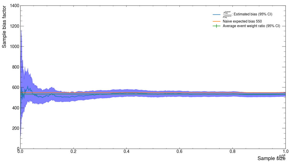
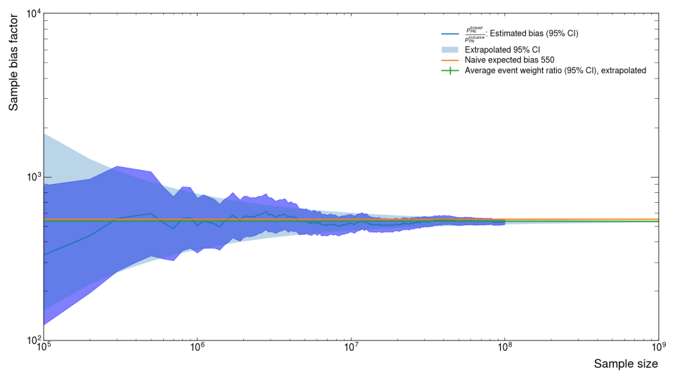
Photon-Nuclear Re-sampling
Often we want to not only require there to be a photon-nuclear interaction in the Ecal, but we also want that photon-nuclear interaction to produce a specific type of interaction (usually specific types of particles and/or how energetic those particles are) -- known as the "event topology".
In order to support this style of sample generation, ldmx-sw is able to be configured such that when the PN interaction is happening, it is repeatedly re-sampled until the configured event topology is produced and then the simulation continues. The estimate \(W\) ends up being a slight over-estimate for samples produced via this more complicated process. Specifically, a "Kaon" sample where there is not an explicit biasing of the photon-nuclear interaction but the photon-nuclear interaction is re-sampled until kaons are produced already shows difference between the "true" value for \(C\) and our two short-hand estimates from before (image below).
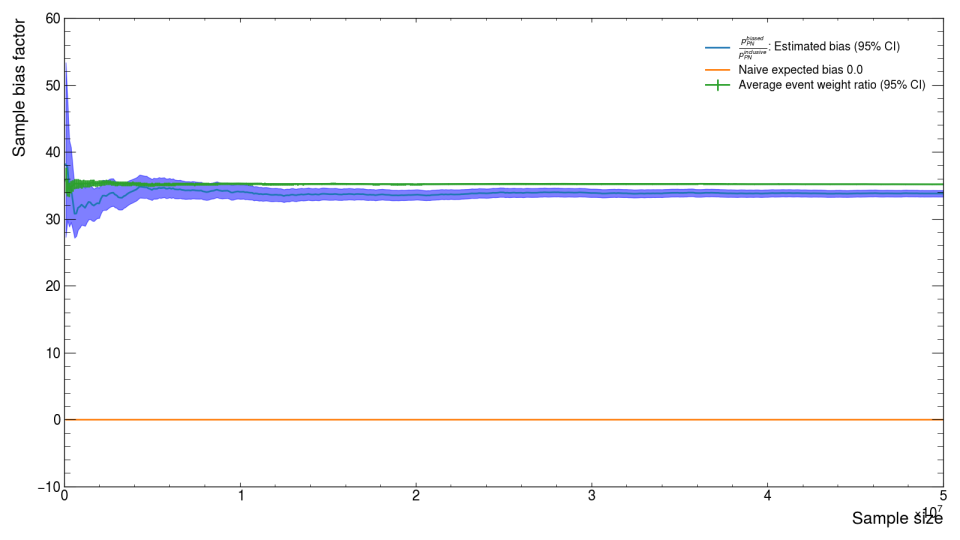
The overly-simple naive expected bias \(B\) is wrong because there is no biasing, but the average event weight ratio estimate \(W\) is also wrong in this case because the current (ldmx-sw v4.5.2) implementation of the re-sampling procedure updates the event weights incorrectly. Issue #1858 documents what we believe is incorrect and a path forward to fixing it. In the meantime, just remember that if you are using this configuration of the simulation, the estimate for the EoT explained above will be slighly higher than the "true" EoT. You can repeat this experiment on a medium sample size (here 5e7 = 50M events) where an inclusive sample can be produced to calculate \(C\) directly.
ECal
Software-related physics topics for the LDMX Electromagnetic Calorimeter (ECal).
Layer Weights
As a sampling calorimeter, the ECal needs to apply weights to all of the energies it measures in order to account for the energy "lost" from particles traversing material that is not active or sensitive. The ECal has sensitive silicon layers that are actually making energy measurements while the rest of the material (tungsten plates, cooling planes, printed circuit boards "PCB") are here treated as "absorber".
Reconstructing the amount of energy deposited within a cell inside the sensitive silicon is another topic, largely a question of interpreting the electronic signals readout using our knowledge of the detector. This document starts with the assumption that we already have an estimate for the amount of energy deposited in the silicon.
I am being intentionally vague here because the estimate for the energy deposited
in the silicon can be retrieved either from the EcalRecHits or the EcalSimHits.
The simulated hits exclude any of the electronic estimation and so are, in some
sense, less realistic; however they could be used to assign blame to energies within
the ECal which is helpful for some studies.
The estimated energy deposited in the silicon is stored in different names in these two classes.
amplitude_member variable ofEcalHit(getAmplitude()accessor in C++)edep_member variable ofEcalSimHit(getEdep()accessor in C++)
Our strategy to account for the absorbing material is to calculate a scaling factor \(S\) increasing the energy deposited in the silicon \(E_\text{silicon}\) up to a value that estimates the energy deposited in all of the absorbing material in front of this silicon layer up to the next sensitive silicon layer \(E_\text{absorber}\). This strategy allows us to keep the relatively accurate estimate of the energy deposited in the silicon as well as avoids double counting absorber layers by uniquely assigning them to a single silicon sensitive layer.
\[ E_\text{absorber} \approx S E_\text{silicon} \]
We can estimate \(S\) by using our knowledge of the detector design and measurements of how much energy particles lose inside of these materials. Many of the measurements of how much energy is lost by particles is focused on "minimum-ionizing particles" or MIPs and so we factor this out by first estimating the number of MIPs within the silicon and then multiplying that number by the estimate energy loss per MIP in the absorbing material.
\[ S = L / E_\text{MIP in Si} \quad\Rightarrow\quad E_\text{absorber} \approx L \frac{E_\text{silicon}}{E_\text{MIP in Si}} \]
The \(L\) in this equation is what the layer weights stored within the software represent. They are the estimated energy loss of a single MIP passing through the absorbing layers in front of a silicon layer up to the next silicon layer.
Calculating the Layer Weights
Calculating the Layer Weights
The Detectors/util/ecal_layer_stack.py
python script calculate these layer weights as well as other aspects of the ECal detector design.
It copies the \(dE/dx\) values estimated within the PDG for the materials within our design
and then uses a coded definition of the material layers and their thicknesses to calculate
these layer weights as well as the positions of the sensitive layers.
Using this estimate for the energy deposited into the absorbing material, we can combine it with our estimate of the energy deposited into the sensitive silicon to obtain a "total energy" represented by a single hit.
\[ E = E_\text{absorber}+E_\text{silicon} \approx L E_\text{silicon} / E_\text{MIP in Si} + E_\text{silicon} = \left(1 + \frac{L}{E_\text{MIP in Si}}\right) E_\text{silicon} \]
Second Order Corrections
Second Order Corrections
From simulations of the detector design, we found that this underestimated the energy of showers
within the ECal by a few percent, so we also introduces another scaling factor \(C\)
(called secondOrderEnergyCorrection in the reconstruction code) that multiplies this total
energy.
\[ E = C \left(1 + \frac{L}{E_\text{MIP in Si}}\right) E_\text{silicon} \]
This is helpful to keep in mind when editing the reconstruction code itself, but for simplicity and understandability if you are manually applying the layer weights (e.g. to use them with sim hits), you should not use this second order correction (i.e. just keep \(C=1\)).
Now that we have an estimate for the total energy represented by a single hit, we can combine energies from multiple hits to obtain shower or cluster "features".
Applying the Layer Weights
In many cases, one can just use the energy_ member variable of the EcalHit class to get
this energy estimate (including the layer weights) already calculated by the reconstruction;
however, in some studies it is helpful to apply them manually. This could be used to study
different values of the layer weights or to apply the layer weights to the EcalSimHits
branch in order to estimate the geometric acceptance (i.e. neglect any electronic noise and
readout affects).
This section focuses on how to apply the layer weights within a python-based analysis
which uses the uproot and awkward packages. We are going to assume that you (the
user) have already loaded some data into an ak.Array with a form matching
N * var * {
  id: int32,
  amplitude: float32
  ... other stuff
}
The N represents the number of events and the var signals that this array has a
variable length sub-array. I am using the EcalHit terminology (i.e. amplitude
represents the energy deposited in just the silicon), but one could use the following
code with sim hits as well following a name change. You can view this form within
a jupyter notebook or by calling show() on the array of interest.
Loading Data into ak.Array
Loading Data into ak.Array
Just as an example, here is how I load the EcalRecHits branch from a pass named
example.
import uproot
import awkward as ak
f = uproot.open('path/to/file.root')
ecal_hits = f['LDMX_Events'].arrays(expressions = 'EcalRecHits_example')
# shorten names for easier access, just renaming columns not doing any data manipulation
ecal_hits = ak.zip({
    m[m.index('.')+1:].strip('_') : ecal_hits.EcalRecHits_valid[m]
    for m in ecal_hits.EcalRecHits_example.fields
})
From here on, I assume that the variable ecal_hits has a ak.Array of data
with a matching form.
Obtain Layer Number
First, we need to obtain the layer number corresponding to each hit. This can be extracted from the detector ID that accompanies each hit.
ecal_hits["layer"] = (ecal_hits.id >> 17) & 0x3f
This bit shifting nonsense was manually deduced from the
ECalID source code
and should be double checked.
The layers should range in values from 0 up to the number
of sensitve layers minus one (currently 33).
If you are running from within the ldmx-sw development or production container
(i.e. have access to an installation of fire), you could also do
from libDetDescr import EcalID
import numpy as np
@np.vectorize
def to_layer(rawid):
    return EcalID(int(rawid)).layer()
to use the C++ code directly. This is less performant but is more likely to be correct.
Efficiently Broadcasting Layer Weights
Now, the complicated bit. We want to efficiently broadcast the layer weights
to all of the hits without having to copy around a bunch of data. awkward
has a solution for this: we can use
IndexedArray
with the layer indices as the index and
ListOffsetArray
with the offsets of the layers to get an ak.Arraythat presents the layer
weights for each hit without having to copy any data around.
First, store the layer weights in order by the layer they correspond to. This is how the layer weights are stored within the python config and so I have copied the v14 geometry values below.
layer_weights = ak.Array([
    2.312, 4.312, 6.522, 7.490, 8.595, 10.253, 10.915, 10.915, 10.915, 10.915, 10.915,
    10.915, 10.915, 10.915, 10.915, 10.915, 10.915, 10.915, 10.915, 10.915, 10.915,
    10.915, 10.915, 14.783, 18.539, 18.539, 18.539, 18.539, 18.539, 18.539, 18.539,
    18.539, 18.539, 9.938
])
Then we use the special arrays linked above to present these layer weights as if there is a copy of the correct one for each hit.
layer_weight_of_each_hit = ak.Array(
    ak.contents.ListOffsetArray(
        ecal_hits.layer.layout.offsets,
        ak.contents.IndexedArray(
            ak.index.Index(ecal_hits.layer.layout.content.data),
            layer_weights.layout
        )
    )
)
Applying Layer Weights
Now that we have an array that has a layer weight for each hit, we can go through the calculation described above to apply these layer weights and get an estimate for the total energy of each hit.
mip_si_energy = 0.130 #MeV - corresponds to ~3.5 eV per e-h pair <- derived from 0.5mm thick Si
(1 + layer_weight_of_each_hit / mip_si_energy)*ecal_hits.amplitude
If you are re-applying the layer weights used in reconstruction, you can
also confirm that your code is functioning properly by comparing the array
calculated above with the energies that the reconstruction provides alongside
the amplitude member variable.
# we need to remove the second order correct that the reconsturction applies
secondOrderEnergyCorrection = 4000. / 3940.5 # extra correction factor used within ldmx-sw for v14
ecal_hits.energy / secondOrderEnergyCorrection
Instructions for how to do visualization with OpenGL (no GUI)
This tutorial was written for ldmx-sw v4.6.4 and contains features not available before that version
One of Geant4’s most reliable visualizers throughout the years, OpenGL (or OGL) is a fast, powerful, yet relatively low-resource rendering program. Despite these advantages, there are two major disadvantages. Firstly, out-of-the-box, it only supports command-line arguments for instructions. Perhaps in a future upgrade we can build Geant4 with Qt enabled so we can provide at least a basic GUI. Secondly, Geant4-specific documentation/tutorials are sparse and have mostly been taught in-person at Geant4 workshops etc. These make it a less attractive choice for visualization, but nevertheless, it’s what is currently working in ldmx-sw.
Basic visualization
g4-vis can be accessed with denv or with just. There is a required
argument (the detector.gdml file for the geometry you wish to
visualize) and an optional argument for a macro file, explained later.
As a concrete example (beginning from the base ldmx-sw directory):
denv g4-vis install/data/detectors/ldmx-det-v15-8gev/detector.gdml
or
just g4-vis install/data/detectors/ldmx-det-v15-8gev/detector.gdml
The detector.gdml file is our gateway to all of the detector’s
sub-components. Take a look in this file, and you’ll see that it loads
(most of) the other .gdml files in this directory one by one. This is
what they call a ‘module’ implementation in GDML. This works so long
as none of the module boundaries are intersecting i.e. the modules are
not physically touching each other. You can even place modules inside
other modules, so long as the parent module fully contains the child
module (again, no boundaries crossing). We’ll cover how to examine
individual components in a later section.
You may notice when you run g4-vis, you get dropped at a command
line interface (CLI). To actually see the geometry you just loaded,
you’ll have to open a viewer screen:
/vis/open OGLIX
Now we have a black screen! Hooray! Let’s populate it with our loaded geometry:
/vis/scene/create
/vis/scene/add/volume
/vis/sceneHandler/attach
The first command creates a new ‘scene’ for OGL. This is an internal instance of a geometry. Multiple scenes can be open at once and switched between, but this is frankly unnecessary functionality so we’ll ignore it from here on in.
The next line adds the ‘volume’(s) i.e. the components to be visualized. By providing no additional arguments, it loads everything into the current scene by default. Again, we’ll cover how to load individual components/modules later.
The final line simply connects your active scene to the viewer, using the ‘scene handler’ intermediary. If I were designing OpenGL, viewers and scenes would be the same thing, especially considering you can open multiple viewers with very little overhead, and we could eliminate two abstractions. Sadly that is not the case.
Navigating the geometry
Navigating the geometry using a CLI isn’t ideal, but it can be manageable, especially with a multi-screen setup. We only need a few commands for navigation; the craft is in knowing how to use them creatively to get the rendering you desire.
The visualization starts centered at the origin point (0,0,0), which in most geometries is the target, and with the viewing angle set to phi=0, theta=0. This is equivalent to standing at the downstream end of the beamline, near the beam dump, and looking backwards along the beam trajectory through the calorimeters. To view along the beamline from the upstream end, rotate your viewpoint 180 degrees:
/vis/viewer/set/viewpointThetaPhi 180 0
Normally, theta specifies the zenith angle and phi specifies the azimuth angle. However, since we use the Z axis as the beam direction in ldmx-sw, you can consider these definitions to be effectively swapped. You can also use a direction vector to specify your viewing angle. The equivalent to the previous command would be
/vis/viewer/set/viewpointVector 0 0 -1
A word of warning: OGL cannot render a viewpoint directly along the axis it considers to be ‘upward’. I never learned exactly why this is, but I guess it’s probably doing some math behind-the-scenes while rendering, which involves dividing by the deviation from the up direction, resulting in a division by zero. OGL by default considers the Y axis to be ‘up’, so these commands are undefined and will show nothing:
/vis/viewer/set/viewpointVector 0 1 0
/vis/viewer/set/viewpointVector 0 -1 0
/vis/viewer/set/viewpointThetaPhi 90 90
It’s also possible to change the ‘focal point’ of the rendering. This can be useful when inspecting components at different positions along the beam path. For example, in v15, to center your viewpoint at (roughly) the most upstream spot on the geometry, where the magnets begin, you can use
/vis/viewer/set/targetPoint 0 0 -1000 mm
OGL doesn’t do ‘perspective’. It doesn’t matter how close or far away a component is; its size relative to other components in the render will stay the same. However, it’s possible to zoom in closer on the focal point (or further away) by setting the zoom scaling factor. Try for example”
/vis/viewer/zoom 0.5
This will zoom out, making everything effectively twice as small. You can get the zoom back to normal with:
/vis/viewer/zoom 2
Occasionally, navigation will break, or not do quite what you want it to do, or you’ll end up lost and unsure which component of the geometry you’re even looking at. You can always return to the default view (focal point at (0,0,0), zoom 1, viewing angle (0,0)) with:
/vis/viewer/reset
When you’re done with your viewing, simply type ‘exit’ in the CLI to exit.
Loading components
There are two ways to specify which components are visualized. Either can be useful, depending on your needs.
The simpler but maybe less elegant way is to edit the .gdml files
directly, especially detector.gdml. If you delete or comment out one
of the components, it’s removed from the geometry. You can see how to
make GDML comment blocks in the files:
<!--This is an example GDML-style comment and will be ignored when
loading the geometry→
Another word of warning: removing components for visualization
purposes will break ldmx-sw in other ways. For example, if you remove
the hcal.gdml module from detector.gdml so that you can see the
other volumes more clearly, then try to run ldmx-sw, it won’t be able
to load an HCal into the geometry and it will crash.
You can also load individual volumes by specifying their names in the
OGL CLI (recommended). By default, a loaded volume will also display
all ‘nested’ volumes, i.e. volumes fully contained inside it (in
Geant4 geometry terms, we refer to the larger volume as the ‘parent’
and the nested volumes as the ‘daughters’). Each of the modules in
detector.gdml contains one big parent volume, which we often refer
to as the envelope (in case you needed more jargon in your life), so
by specifying this parent volume, you can load individual modules, or
combinations thereof.
With your OGL CLI open and detector.gdml loaded, try typing:
/vis/drawTree
This will display thousands of lines of code. Each line is the name of one of the volumes loaded into our geometry. As an example, the last several lines of the v15 geometry tree look like this:
    "ldmx_magnet_PV":0 "coil_1_vol_PV":0 "coil_2_vol_PV":0
      "shim_right_PV":0 "shim_left_PV":0
      "corner_iron_block_top_left_PV":0
      "corner_iron_block_top_right_PV":0
      "corner_iron_block_bot_left_PV":0
      "corner_iron_block_bot_right_PV":0 "center_iron_block_top_PV":0
      "center_iron_block_bot_PV":0
Notice that the first line has less indentation than the next
lines. The indentations indicate mother-daughter relations. Thus, all
of the lines below ldmx_magnet_PV are daughters of ldmx_magnet_PV,
and by default will be loaded along with it. If you’re in the v15
geometry you can try this yourself:
/vis/open OGLIX
/vis/scene/create
/vis/sceneHandler/attach
/vis/scene/add/volume ldmx_magnet_PV
Notice that we attached the scene to the viewer before even loading
anything! This is fine; the viewer will refresh each time you add
something or make other significant changes. To save you lots of
scrolling, here are the names of the envelope for each module in
detector.gdml as of v15:
tagger_PV
TS_trgt_PV
trig_scint_tagger_PV
recoil_PV
em_calorimeters_PV
hadronic_calorimeter_PV
ldmx_magnet_PV
The ‘_PV’ is added to all of the names automatically by GDML, and
indicates that this is a physical volume. Don’t worry too much about
it - but you do have to include it. If you /vis/scene/add each of
these, you’ll load the entire geometry, just like we did by providing
no arguments to this command. You can also draw the geometry tree of
individual components, for example:
/vis/drawTree TS_trgt_PV
You may notice a : followed by a number for most volume names. This is the ‘copy number’. Often, when iteratively placing volumes, we’ll place the same volume with the same name multiple times. The copy numbers help them to remain logically distinct. If for some reason you’d like to examine a single copy of a volume placed multiple times, simply provide the copy number as a second argument when adding the volume:
/vis/scene/add/volume tspad3_lightpipe_volume_PV 40
This loads only one of the light pipes in TSPad3, the one with copy number 40.
Visualization macros
So far this tutorial has covered using OGL in the CLI. It’s also
possible to write a macro - a set of commands - which can be executed
sequentially. To execute all the commands in a macro file, simply use
(while at the g4-vis CLI):
/control/execute /path/to/macrofile.mac
It's also possible to execute the macro file immediately after loading
the geometry, by giving just the path to the macro as a second
argument:
just g4-vis /path/to/detector.gdml /path/to/macrofile.mac
A few example macro files have been included with this tutorial, to do things such as examining the TSPads in greater detail, rendering the ECal, viewing the entire geometry, and a special example which showcases some of the other tools available in the visualizer.
How to learn more
You can try your luck at googling for OpenGL tutorials. These are often quite old, but the functionality hasn’t evolved much in the past 10 years. There are also books and stuff but I’ve never actually seen one. I don’t know what to tell you for GDML. There’s a manual, but it’s missing a lot of details.
There are two essential commands which can help you learn more about
OpenGL: ls and help. First, let’s re-examine a typical OGL
command:
/vis/viewer/set/targetPoint
You can think of /vis/, /viewer/, and /set/ as directories. This
is just a way of organizing the hundreds of OGL commands
logically. Like a typical directory, you can use ls to see what’s
inside of it:
ls /vis/viewer/set
ls /vis
etc
However, the last part, targetPoint, is not a file. It is still a
command, and almost all commands accept arguments. To learn more about
the functionality and arguments of the command, use help.
help /vis/viewer/set/targetPoint
etc
Technical details that don’t really fit in the rest of the tutorial
but should be written somewhere
A recent PR has ‘fixed’ OGL in ldmx-sw by moving the XSD style sheets
- used by GDML for XML-style formatting - from online to offline
(i.e. local) locations. It seems that for whatever reason, internet
functionality is limited in the current version of ldmx-sw. I wouldn’t
even know where to begin fixing this, so we accrue a bit more tech
debt and work around it. For now, I’ve taken advantage of an existing
piece of the CMakeLists.txt for detectors, which gives absolute paths
to all of the GDML files when compiling ldmx-sw, and used it for the
XSD files as well. This has one major disadvantage in that it requires
the same set of XSD files to exist as copies in each geometry version
directory. So there will be a /path/to/v14/*.xsd and a
/path/to/v15/*.xsd and so on. This can be solved in a future small
PR, in which the .xsd files are in a separate directory and are only
copied once for all geometry versions.
Glossary
Copy - One instance of one volume which has been placed multiple times. For example, a TSPad has 48 identical scintillator bars, so there are 48 copies of the volume for a scintillator bar.
Daughter - A volume entirely surrounded by a larger volume, its ‘parent’.
Envelope - The parent volume of an entire module, containing all its components.
Focal point/focus - The central point of the OpenGL visualization. Defaults to the origin.
GDML - Geometry Description Markup Language, a variant of XML used to describe geometries. Like XML, it’s basically an enormous set of nested parameters, which are logically read and assigned to Geant4 objects during runtime.
Geometry - A general term for all of the volumes in a simulation. Sometimes interchangeable with the term ‘world’, when talking about one specific geometry.
Module - A self-contained collection of volumes. Has one ‘envelope’, a giant parent volume, populated with many daughters. Load several of these to make a complete geometry.
OGL - OpenGL (Open Graphics Library) is a cross-language, multi-platform application programming interface (API) for rendering 2D and 3D vector graphics. I copied this directly from a webpage.
Parent - A large volume which completely encompasses one or more smaller volumes, the daughters.
Scene - an internal instance of a geometry in OpenGL. A scene exists without being displayed until it’s attached to a viewer.
Scene Handler - the intermediary in OpenGL which communicates between the scene and the viewer.
Viewer - a graphical window in OpenGL, used to display the rendered geometry.
Volume - a single object in a geometry, such as one SiPM, one HCal quad bar etc. Interchangeable with ‘component’.
XML - eXtensible markup language. This is a generalized data storage language, with tools to categorize and search for/retrieve data quickly and unambiguously. It’s not very friendly for human readability, and is typically generated and read automatically.
XSD - XML Schema Definition. This is XML’s way of defining a set of rules for parsing and interpreting parameters. GDML is basically just XML with special XSD files designed for geometry reading/writing.
Documentation added by CJ Barton, Lund University, March 2026
Getting Started Developing ldmx-sw
This guide assumes familiarity with the first-time using guide and with the terminal.
Moving from using ldmx-sw to developing ldmx-sw is a common occurrence as issues or missing features are discovered in the course of analyzing the physical results.
Do not fear! We still use containers to share the software and thus
the container runner and denv which you installed to use ldmx-sw
will still be used when developing ldmx-sw.
In fact, after building ldmx-sw yourself, you will still be able
to run denv fire (and similar) commands like before - it will
just use your local, custom build of ldmx-sw rather than the
released version you chose before.
We need a few more tools to help track our changes and share commands that we use regularly.
Make sure git is installed
git is a very common tool used by software developers and so it may already be
available on the system you are using for development.
Even if not (the test below fails), a simple internet search for
install git <your-operating-system> will give you guidance.
- Make sure
gitis installed within WSL on Windows. There are other ways to interact withgiton Windows (e.g. GitBash), but that is not what we want. - On MacOS, the default installation of
gitthat comes with Apple's developer tools does not include thelfssub-command which is required by one of ldmx-sw's dependencies (acts to be specific). Luckily, GitHub has a nice tutorial on how to installgit lfson MacOS.
Both of the commands below should printout a help message rather than a
Command not found error.
git
git lfs
Install just
just has a myriad of ways to be installed, but - like denv - it has
a simple download method that allows
you to get the most recent version on most systems.
For example, we can install just into the same directory where denv is
installed by default.
curl --proto '=https' --tlsv1.2 -sSf https://just.systems/install.sh |\
  bash -s -- --to ~/.local/bin
If the above does not work on your operating system, you can see system specific instructions on the just website
You probably want to enable shell tab-completion with just
which only needs to be done once per installation but will help save typing.
And then you can enable just's tab completion in bash by putting
eval "$(just --completions bash)"
in your ~/.bashrc file. If you are using other shells, make sure to
check which file to write to and what the syntax should be.
You can run the command just within your terminal.
just
Without a justfile already residing within your current directory,
just will printout an error. For example:
$ just
error: No justfile found
justis not technically required in order to develop ldmx-sw. The recipes within thejustfilecan be read with any text editor and you can manually type them into the terminal yourself; nevertheless, that would be a lot more typing and error prone.
Quick Switch to denv+just
No frills, no explanations.
If anything goes wrong, fall back to the more full getting
started guides for using (for details on denv)
or developing (for details on just).
This is targeted towards LDMX contributors who were present
before the transition to denv+just so they already have
a container runner present on their machine.
# install denv into ~/.local
curl -s https://raw.githubusercontent.com/tomeichlersmith/denv/main/install | sh
# install just into the same location
curl --proto '=https' --tlsv1.2 -sSf https://just.systems/install.sh |\
  bash -s -- --to ~/.local/bin
# add just tab completion to your ~/.bashrc
printf '\neval "$(just --completions bash)"\n' >> ~/.bashrc
The denv install script attempts to help you update your ~/.bashrc
so that ~/.local/bin is in your PATH and discoverable by bash as
a program, but you may need to update your PATH manually.
While the justfile defining our shared configuring, building,
testing, etc recipes is on trunk, it may not be on the branch you
are developing on.
There are two solutions to this:
- Update your branch to be based off the new
trunk.
git switch trunk
git pull
git switch -
git rebase trunk
- Just use
denvdirectly in place ofldmx.
denv cmake -B build -S .
denv cmake --build build --target install
# and most of the others
Build and Installing ldmx-sw
There are many intricasies that come with building such a large software project. This chapter is focused on providing guides on how to accomplish this build and more detailes related to it.
This chapter assumes you already finished with everything under "Getting started"
Clone the Software Repository
In a terminal, go to the directory where you will keep all of your LDMX software and run the following command.
git clone --recursive git@github.com:LDMX-Software/ldmx-sw.git
- The
--recursiveflag is very important because there are several necessary parts of ldmx-sw stored in separate git repositories. - The above
cloneuses an SSH connection which requires you to create a GitHub account and connect to it with SSH.
Changing the link after cloning
Changing the link after cloning
If you find yourself with an already cloned copy of ldmx-sw that was cloned with the HTTPS link and you wish to create a new branch and push, you can switch the link of the remote to the SSH version on your machine without having to re-clone.
git remote set-url origin git@github.com:LDMX-Software/ldmx-sw.git
This is especially helpful if you've already made some changes you do not want to lose.
You can see the ldmx-sw software directory in your terminal.
ls
# 'ldmx-sw' is one of the entries printed
cd ldmx-sw
just
# our justfile's default recipe is to printout all the possible commands
Setup the Environment
One of the recipes within our justfile handles initializing a default environment.
just init
- This command downloads the latest development image, so it may take some time (a few minutes) on the first run.
- This command only needs to be done once per clone of ldmx-sw. Look at the other commands available from
justfor changing the environment. - On shared computing clusters, the specific filesystem configuration may not be well suited to downloading the image with the default configuration. For apptainer, be aware that you can move the directory in-which images are stored using the
APPTAINER_CACHEDIRenvironment variable and move the directory in-which the build takes place using theTMPDIRenvironment variable. This is specifically an issue for SLAC's SDF and S3DF which have very small/tmpdirectories (what apptainer uses ifTMPDIRis not defined).- The
justfileupdates the default definition ofAPPTAINER_CACHEDIRto be the parent directory of ldmx-sw, but this may still not be the best location.
- The
You can view the environment configuration from denv.
denv config print
# detail of how the environment is configured
If you see something like "no workspace found", then something went wrong during the environment setup.
Development Cycle
The justfile contains many recipes that are helpful so inspect the output
printed when just is run with no arguments to view some of them.
The default build can be created with
just compile
You can pass CMake variables to the configure command (sanitizer is just an example)
and then build the updated configuration.
just configure -DENABLE_SANITIZER_ADDRESS=ON
just build
For the CLANG compiler with LTO please run
just configure-clang-lto
just build
Often you will want to recompile and run a config script.
just recompFire my-config.py [config args ...]
Running the test suite is done with
just test
Shared Computing Clusters
Building, installing, and running ldmx-sw on shared computing clusters is largely similar to how it is done on personal laptops; however, there are special considerations to be made that can make it functional.
All of the clusters LDMX has access to are focused on using singularity (or its newer brand apptainer), so these comments are focused on this runner.
Image Cache and Build Directories
The ldmx-env.sh script moves the singularity cache directory to be within the LDMX_BASE
directory. This is done to avoid filling a user's home directory (the default cache location)
with large image layers. Besides the cache directory, singularity also uses a temporary
directory for constructing the final image file. On some clusters (notably SDF), the default
temporary directory is not large enough to fully construct this image file and so it may
need to be moved.
SINGULARITY_CACHEDIRorAPPTAINER_CACHEDIRcan be used to change the location of the image layer cache for singularity/apptainer.TMPDIRis inspected by singularity/apptainer for the temporary build location. Change this variable if the build is failing due to disk space issues.
Shared Images
We do not run containers that modify the original image, so shared computing clusters could share a lot of space by have image files be centrally produced and then users all share the same image files so they don't have to have their own copy.
Currently, there is not a mechanism within the ldmx-env.sh script to direct the ldmx
command to an area with shared images, but we can circumvent this issue easily with
symlinks. Below, I outline a method to keep all of the LDMX images within one shared
directory that users can use instead of their own copies.
If ldmx-env.sh evolves to support moving the image storage location
(for example by refactoring to use denv instead
Issue #1232
which does support this for singularity/apptainer runners),
we could put the ldmx/dev repository onto the CVMFS unpacked.cern.ch
repository
which would make the images available via CVMFS saving disk space
and network bandwidth.
Let LDMX_SHARED_IMAGES be an environment variable storing the full path to a directory
that we want to share images in. A single person with access to the cluster and to this
directory should be the builder of these images, everyone else on this cluster is called
a user.
Builder Steps
Whenever there is a new release of the container image, build it and update the latest symlink.
cd ${LDMX_SHARED_IMAGES}
apptainer build ldmx_dev_vX.X.X.sif docker://ldmx/dev:vX.X.X
ln -sf ldmx_dev_vX.X.X.sif ldmx_dev_latest.sif
This mimics the naming of the *.sif files that is done within the ldmx command
and avoids copying the latest image, preferring instead to just symlink from the _latest.sif
name to the copy of that tag.
Builders will need to be slightly more familiar with apptainer/singularity in
order to issue this command. They may need to change the cache directory with APPTAINER_CACHEDIR
or the build directory with TMPDIR depending on how much space is available to them
on their cluster.
User Steps
In order to use a directory of shared images, one just needs to remember to symlink
the available images into their LDMX_BASE area before sourcing the environment script.
ln -sft . ${LDMX_SHARED_IMAGES}/*sif
. ldmx-sw/scripts/ldmx-env.sh
This informs ldmx-env.sh that the images are already available since they are in the
LDMX_BASE directory with the correct names and so ldmx will only pull down and make
a copy of an image if it wasn't in the shared images location.
Since the symlinking procedure is rather quick, you could probably just fold this into
every source you do to avoid any forgetfulness.
# in .bashrc
export LDMX_BASE=/full/path/to/ldmx/base
export LDMX_SHARED_IMAGES=/another/path/to/shared/images
ldmx-env() {
  # make sure list of already downloaded images is up-to-date
  ln -sft ${LDMX_BASE} ${LDMX_SHARED_IMAGES}/*.sif || return $?
  # setup ldmx environment
  . ${LDMX_BASE}/ldmx-sw/scripts/ldmx-env.sh || return $?
  # add a [ldmx] tag to the PS1
  export PS1="[ldmx] $PS1"
  # delete this function to avoid double-environment
  unset -f ldmx-env
}
Updating ldmx-sw
This page is helpful for those coming back to ldmx-sw and wishing to update there local copy of it. It can also be a helpful guide for anyone interesting in debugging ldmx-sw since often it is helpful to start with the most recent ldmx-sw.
We can update ldmx-sw through three main stages. These stages are not necessarily connected (i.e. you could update the code and re-build without changing the environment if desired).
Update Environment
There is a just recipe that updates the environment on your machine.
just pull dev latest
The pull command informs just to download the latest image no matter what
(The more common use command will only spend time downloading if the image is
not available.)
The latest tag is one tag that evolves with the image as new versions are built.
If you wish to avoid accidentally upgrading your environment, you are encouraged
to use specific versions of the image (e.g. just use dev 4.2.0).
Update Source Code
Updating the source code of ldmx-sw mostly amounts to using various git comands
to download the updates other developers have uploaded to GitHub.
First, we switch to the main branch of ldmx-sw trunk.
Even if you are on a different branch, it will be best to first update your local
trunk before trying to update your different branch.
git switch trunk
Now pull down the updates from GitHub.
git pull origin trunk
Finally, make sure any submodules that were updated or newly introduced are also updated along with the change in source code.
git submodule update --init --recursive
You can avoid this last step by updating your local git configuration
to (effectively) call this command after other commands like git pull.
git config submodule.recurse true
This is available in Git versions >= 2.14
If you are on a different branch (and want to carry your changes with you),
you can now go back to that branch and re-apply your updates on top of the
new trunk. This process is called "rebasing" and can lead to conflicts if the
files you changed are the same as ones changed on trunk. For small changes
or additions (e.g. adding a new processor for an analysis), this can be done
with ease and it will make comparing your developments to what is on trunk
easier.
git switch my-branch
git rebase trunk
Fully Clean Re-Build
Cleaning the source tree is necessary to remove any files generated during the building
process. The programs we use to configure (CMake) and build (make) our software do a pretty
good job of automatically re-building files if the source files change, but we have some
custom configuration that does not follow this protocol and sometimes leads to errors.
To avoid these errors, it is helpful to remove all generated files and start a new
build "clean" (or from scratch). The following git commands remove all files that
are not being tracked by git (and thus we assume are generated files).
git clean -xfd
git submodule foreach --recursive git clean -xfd
If you want to persist some files that are within the ldmx-sw directory and are not
being tracked by git (for example, some data files), then you will need to at minimum
delete the build and install directories and clean out the generated files from the Framework
directory.
rm -r build install
git -C Framework clean -xfd
If you are updating from a version of ldmx-sw newer that v3.3.4, then the generated files that used to be written outside of the build directory are being written inside now. This means you can remove all generated files simply by
rm -r build install
# same as 'just clean' after v4.1.0
and without any git clean commands.
The final build and install steps are similar to the past ones. Just note that they will take longer since the build is starting from scratch.
denv cmake -B build -S .
denv cmake --build build --target install
# same as 'just configure build' after v4.1.0
ldmx-sw Framework Structure
ldmx-sw is organized into "modules" that contain related code, the Framework module
is of particular importance since it defines the core processing interfaces and handles
reading/writing data from/to the ROOT files.
The overall flow of a successful execution of fire goees through two stages.
- Configure - run the provided Python script and then extract the run configuration from the Python objects that were created when the script was run.
- Run - execute the configured run. The
framework::Processclass is the main object that handles the execution.
Where is the main?
Where is the main?
Many developers, especially those who are more familiar with C++, will want to know
where the fire executable is defined.
fire is defined within Framework/app/fire.cxx and this file reveals the overall
flow of the program.
How does Python get run?
How does Python get run?
We launch Python from within our C++ program by
embedding Python.
In the configuration area of Framework, you'll see may of these calls to Python's
C interface (like Py_InitializeEx() for example).
Why use Python for configuration?
Why use Python for configuration?
It's easier than maintaining our own language for configuration.
The sheer number of configuration parameters makes it necessary to organize them based on which parts of the software they correspond to. This then necessitates some kind of configuration language in order to instruct the software of the values for the multitude of parameters.
Geant4 has a similar issue and chose to develop their own configuration
language -- search "Geant4 macro commands" online to see what it looks like.
Besides being a huge technical debt in order to maintain such a language,
we also then lose all of the helpful benefits of running Python.
Users can use Python libraries (like sys, os, and argparse) to
allow for their configuration to be "smarter" and inspect command line
arguments as well as environment variables.
We can implement checks on the configuration in Python
in order to catch any configuration issues as early as possible.
We require ldmx-sw to do a lot of different tasks and the Framework is present to make sure those different tasks can be developed on top of a known structure. The following pieces of Framework helps introduce the vocabulary as well as explain how they are used.
Each of these classes in C++ has a "mirror" Python class that is used to configure it. While the Python configuration class is not strictly necessary for the configuration system to function as intended, it is very helpful to keep parameters organized and have the configuration understandable.
A C++ producer that is declared like
class MyProducer : public framework::Producer {
would have a mirror python configuration class defined like
class MyProducer(ldmxcfg.Producer):
This mirroring helps point out that all the configuration parameters
within the Python MyProducer are meant to be used by the C++ MyProducer.
Processor
A processor is the main object that developers of ldmx-sw interact with. They are used to create the objects within an event ("Producer") and analyze those objects ("Analyzer"). A processor is given access to the event where it can access the event objects from an input file or produced by earlier producers. They can also be used to fill histograms which are stored into the output histogram file and provided "storage hints" that can be used to decide if a specific event should be written into the output event file.
Conditions
A "condition" is an object that is the same for many events in sequence (like a table of electrical gains or the "geometry" of the detector). Conditions are provided by "Conditions Object Providers" that can be written by ldmx-sw developers. These providers only construct the conditions themselves when the condition is requested by a processor. They take information from the current event to see how to configure the condition that is being constructed and how long the constructed condition is valid for ("interval of validity" or IOV). The Framework then can come back to the provider to construct a new condition if the condition that was previously provided is not valid anymore.
Transition to ldmx-sw v4
If you don't have a branch of ldmx-sw that you wish to update, the easiest way to update ldmx-sw to v4 is with a new clone.
rm -rf ldmx-sw # are you SURE you have no changes? We are deleting everything now...
git clone --recursive git@github.com:LDMX-Software/ldmx-sw.git
Make sure your container image is newer than v4 as well.
just init pull dev latest
Before the major release v4, ldmx-sw contained a lot of git submodules.
They were introduced to try to help improve the developing workflow, but
they ended up being an impedance for how we develop ldmx-sw and so were
removed. Changing a git submodule into a normal subdirectory is a highly
technical change that, while it doesn't change the source code, significantly
alters how users interact with the source code via git.
Goals
This documentation page is here to help users update their local copy of ldmx-sw from before the v4 transition to after the v4 transition.
- The target audience are those less familiar with
git - We aim to avoid manually re-writing changes
The process described here is similar to "squashing" all of the changes on a branch into one commit. While the history of a branch is sometimes helpful when trying to understand the code, carrying the history through this transition is a complicated process that is non uniform. Discarding the history of a branch in the way described here will also discard any previous committers or authors of the changes. Assuming the branch has just been edited by an individual developer, squashing the changes into one commit and discarding the history is an acceptable procedure in most cases. If you have a branch with multiple authors or a history you'd like to preserve, please reach out. We can talk about trying to recover the history while updating the branch.
With the introduction out of the way, let's get started.
Step 1: Align branch with ldmx-sw v3.4.0
The last release before the de-submodule transition was v3.4.0, and in order for the update to work as described below, your branch must first be "aligned" with this version of ldmx-sw.
# make sure you have access to the tags of ldmx-sw
git fetch --tags
# merge the v3.4.0 tag into your branch
# https://stackoverflow.com/a/3364506
git merge -X theirs v3.4.0
# check that the resulting diff contains your changes
git diff v3.4.0
Step 2: Prepare to Cross Boundary
The submodule to no-submodule transition is one that git struggles with, especially when
going "backwards" (i.e. going from a branch after the transition to one from before the transition),
so it is easiest to make a new clone and rename your old clone to emphasize
that it is the old one.
mv ldmx-sw old-ldmx-sw # rename old clone
git clone --recursive git@github.com:LDMX-Software/ldmx-sw.git # get new clone
Then create a new branch in the new clone that has the same name as the branch you want to update.
git -C ldmx-sw switch --create my-branch
If you see any warnings or errors, that means a local copy of my-branch already exists in the
new clone of ldmx-sw. This should not happen.
Step 3: Cross Transition Boundary
The basic idea behind this procedure is to write your changes into a file (called a "patch" file) and then re-apply those changes onto the new version of ldmx-sw. The actual procedure for doing this depends on where your changes are, so the specifics of creating and applying these patch files are separated into categories depending on where your changes are. All of the categories assume that you have done Steps 1 and 2 above.
No Changes
No Changes
Your branch doesn't have any changes (or you were just running a locally-compiled version of ldmx-sw trunk).
This is the easiest case and I would just suggest to remove the old clone of ldmx-sw equivalent to the TLDR at the top of the page.
rm -rf old-ldmx-sw # are you SURE you have no changes you want to keep?
Changes only in ldmx-sw (and nothing in submodules)
Changes only in ldmx-sw (and nothing in submodules)
The changes you made are not in any of the submodules (i.e. you haven't changed files within
cmake, Conditions, SimCore, Tracking, Trigger, Framework, MagFieldMap, TrigScint,
Ecal, or Hcal).
This means that the changes you've made can be re-applied to the post-transition ldmx-sw with relative ease since their location hasn't changed.
cd old-ldmx-sw
git diff v3.4.0 > ../my-branch.patch
cd ../ldmx-sw/
git apply ../my-branch.patch
Changes within a submodule
Changes within a submodule
The basic idea is the same, but since the path to the files being changed also changes, we need to use an extra argument when applying the changes to the new clone of ldmx-sw.
Call the submodule your changes are in submodule (for example, if you have edits in Ecal,
the replace submodule with Ecal in the commands below), then the following lines
will re-apply the changes currently within the submodule in the old-ldmx-sw clone
of ldmx-sw onto the same files within that directory of the new ldmx-sw clone.
cd old-ldmx-sw/submodule
git fetch
# the following just gets the default branch of the submodule
# you could equivalently just look it up on GitHub
sm_main="$(git -C ${sm} remote show origin | sed -n '/HEAD branch/s/.*: //p')"
git diff origin/${sm_main} > ../../my-branch.submodule.patch
cd ../../ldmx-sw
git apply --directory=submodule ../my-branch.submodule.patch
Changes across many submodules or in both ldmx-sw and a submodule
Changes across many submodules or in both ldmx-sw and a submodule
You can combine the two procedures above with the following additional notes.
Follow the changes within a submodule procedure for each submodule. This is pretty self-explanatory, you could even create a different commit on the newly updated branch for each submodule if you want.
Exclude any submodule changes when following the ldmx-sw only procedure. This is a bit more complicated. If you know which files are different, the easiest way to avoid including the submodule changes is to explicitly list the files in ldmx-sw that have changed.
git diff v3.4.0 <list of changed files> > ../ldmx-sw-only-changes.patch
You could also remove the chunks of the .patch file manually with a text editor, but that is
more difficult and requires more familiarity with the syntax of patch files.
Step 4: Check and Commit
For this final step, we are in the new clone ldmx-sw and we've already run git apply
(according to the commands in Step 3) so that the changes from the old branch have been applied.
Make sure to check that your edits have been applied as you've desired and they work as you expected. This includes (but is not limited to):
- Look through the output of
git statusto make sure the files you wanted to change are changed - Look through the output of
git diffto make sure the files changed how you wanted them to change - Recompile ldmx-sw with your changes (if they were compiling before the transition)
- Rerun and re-test the changes (if they were running and passing tests before the transition)
Now that the updates have been properly checked, we can add the changes we've made and commit them to the new branch in the new clone of ldmx-sw.
git add <files-that-you-changed>
git commit
Make sure to write a detailed commit message explaining ALL of the changes you've made (not just the most recent ones). Remember, the old commits and their messages will be deleted!
I am pausing here to remind you to double check that your changes are what you expect
and want.
Once we run the next command, the old version of my-branch on GitHub will
be deleted and replaced with the new version.
git push --force --set-upstream origin my-branch
I am pausing here to remind you to triple check that your changes are what you expect
and want. Once we run the next command, the old version of my-branch on your computer
will be deleted.
Only run this next command when you are done transitioning all of your branches
if you have multiple branches.
cd ..
rm -rf old-ldmx-sw
Extra Notes
When attempting to go from after the transition to before the transition, git
struggles to handle the recursive submodule structure that we had in ldmx-sw. The first
submodule that has this issue is SimCore so you'll see an error like the following
fatal: could not get a repository handle for submodule 'SimCore'
In this case, I would suggest that you simply make a separate clone of ldmx-sw.
The --branch argument to git clone allows you to clone a specific branch or tag
rather than the default one (trunk) so you can have a clone of a specific branch or tag
that is from before the transition.
git clone --branch <name> --recursive git@github.com:LDMX-Software/ldmx-sw.git
If you are observing a compilation issue involving std::string_view
after updating your to ldmx-sw v4, you are probably observing the incompatibility
between ldmx-sw >= v3.3.5 and the container image < v4.
The solution for this is to update the image you are running to build ldmx-sw
to one that is >= v4.0.0. The simplest way to do this is just to update to the
latest image with just pull dev latest, but you can also simply make sure
you are using an image that was create after June 22, 2023 (when v4.0.0 was
built and pushed to DockerHub).
Tracking the Performance of ldmx-sw
With v1.4.0 of Framework, rudimentary performance tracking is available to all users of Framework. This first release only tracks the time of various components leaving more complicated measurements (e.g. memory consumption) for later.
Performance is tracked in an opt-in basis and is stored within the output histogram file underneath a directory named "performance". In order to track performance, you must update your config file with the following data.
# p is the ldmxcfg.Process object already constructed
p.histogramFile = 'performance.root' # only necessary if not already being used
p.logPerformance = True
The performance measurements are measuring how long a specific callback took as well as some additional timing measurements.
absolute: timing how long the entire process took to run (ignoring the configuration time)onProcessStart: how longonProcessStarttookonProcessEnd: how longonProcessEndtookonFileOpen: how long the lastonFileOpentookonFileClose: how long the lastonFileClosetookbeforeNewRun: how long the lastbeforeNewRuntookonNewRun: how long the lastonNewRuntookby_event: timing of each processing call took for each event
Some callbacks (the File and Run ones) can be called multiple times during
reconstruction mode. The performance tracking software only stores the last
measurement since it is focused on measuring production runs.
Future developments to measure every call to these functions would not be difficult, but would require some complication of the data schema.
Each of these measurements are further separated into the different processors in the sequence by the name given to the processor in the configuration. A special name "__ALL__" is used for a measurement that times how long all of the processors in the sequence took for that callback. The performance measurements are stored in the output histogram file under the following schema. All timing measurements use the framework::performance::Timer class.
- performance/      # TDirectory holding all performance data
  - absolute        # Timer for all
  - onProcessStart/ # TDirectory holding onProcessStart data
    - <processor>   # Timer for processor named <processor>
    - ...
    - __ALL__       # Timer wrapping all processor's onProcessStart calls
  - ... other non-by-event call-backs follow same structure
  - by_event/
    - <processor>   # branch holding instances of Timer for processor named <processor>
    - ...
    - __ALL__       # wrapping all processor's producer or analyze calls
    - completed     # boolean signalling if event was completed (true) or aborted (false)
Accessing this schema is not too difficult, but as an example, I've included some python
snippets below using uproot that just prints the performance data from the input
file to the terminal.
"""load a file and print the performance data"""

import uproot
import sys
import json

class ReprEncoder(json.JSONEncoder):
    """if JSON can't serialize it, just use its repr string"""
    def default(self, obj):
        try:
            return super().default(obj)
        except TypeError:
            return repr(obj)


with uproot.open(sys.argv[1]) as f:
    print('absolute')
    t = f['performance/absolute'].members
    print(t['duration_'], t['start_time_'])
    for callback in [
        'onProcessStart', 'onProcessEnd',
        'onFileOpen','onFileClose',
        'beforeNewRun', 'onNewRun'
    ]:
        print(callback)
        for name, timer in f[f'performance/{callback}'].items():
            print('  ', f'{name:10s}', f'{timer.members["duration_"]:.3e}', timer.members['start_time_'])

    t = f['performance/by_event']
    # use recursive=False so that the branches remain structured into their Timers
    # you can also remove the expressions argument which will just return an unstructured set of data
    events = t.arrays(expressions=t.keys(recursive=False), library='np')
    print(json.dumps(events, cls=ReprEncoder, indent=2))
Container-Software Compatibility
Often we need to introduce new dependencies in order to do new things in our software. Occasionally we make mistakes with these dependencies and need to fix how they are configured or installed. Both of these reasons cause some compatibility issues where all versions of ldmx-sw are not necessarily buildable by all versions of the container.
The "container image" is version controlled in its repository LDMX-Software/dev-build-context. If you are interested in looking for which minimum version of the container has your desired dependency, you should look through the releases of the container.
The ldmx-sw versions are documented in the "releases" of the LDMX-Software/ldmx-sw repository, but you should also read these versions as inclusive of branches that are based off of them. For example, if you made a branch when ldmx-sw was version 3.0 you may not be able to use a container that is incompatible with ldmx-sw version 3.0 (i.e. you might need to introduce updates to later versions of ldmx-sw onto your branch to use a newer container).
The ordering of versions follows semantic versioning (i.e. order by major version, then minor version, then patch).
This compatibility table is manually written and not everything has been directly tested. Updates to this document from your personal experience are welcome and encouraged.
For each range of versions of compatibility, we've written a table corresponding to different container versions required for different build configurations of ldmx-sw. This was done since many new features that require new dependencies are first introduced as opt-in features. Below, I've written a table allowing you to know what I mean by certain build configurations.
| build config | meaning |
|---|---|
| default | No parameters given to cmake besides necessary ones |
| no testing | disable testing which is enabled by default1 |
| force legacy onnx | ldmx-sw's CMake code for finding ONNX didn't work well and so it needs to be modified slightly2 |
| sanitizers | enable one or more of the sanitizers, cmake: -DENABLE_SANITIZER_*=ON |
| detector id bindings | enable detector ID python bindings, cmake: -DBUILD_DETECTORID_BINDINGS=ON |
| patch cmake | need to do both no testing and force legacy onnx |
| header patch | transitioning to a newer compiler then required a few more headers to be included3 |
| include lorentz vector | add Math/GenVector/LorentzVector.h and Math/Vector4Dfwd.h to inclusions in Ecal/IntermediateCluster.h |
Currently in ldmx-sw, there isn't a command-line option to disable the
testing so one must comment out the build_test() line in ldmx-sw/CMakeLists.txt.
Using a version of software without any testing being built is not a good idea,
unless you need to stay on an old version for a good reason it would be much
better to update your branch to a newer version of ldmx-sw and update the container
to the newest version as well.
Forcing legacy onnx is relatively simple and can be done by commenting out the
find_path call within the ldmx-sw/cmake/FindONNXRuntime.cmake file. This
prevents CMake from finding the system install in newer containers.
The specific headers needed vary depending on the version you are attempting to build. You can either look at the patch files for different versions or simply follow the compiler's instructions for including the appropriate headers.
Pre-v3.0.0
No containers have been studied for older versions of ldmx-sw. Although, there was a patch-release of v1.7.0 so that it could run in an image.
>=v3.0.0 and < v3.1.1
| build config | image version |
|---|---|
| default | < v4.0.0 |
| patch cmake | >= v4.0.0, < v5.0.0 |
>=v3.1.1 and < v3.1.12
| build config | image version |
|---|---|
| default | < v4.0.0 |
| patch cmake | >= v4.0.0, < v5.0.0 |
| with sanitizers | > v3.2, < v5.0.0 |
>= v3.1.12 and < v3.2.4
| build config | image version |
|---|---|
| default | < v4.0.0 |
| patch cmake | >= v4.0.0, < v5.0.0 |
| with sanitizers | > v3.2, < v5.0.0 |
| with detector id bindings | > v3.3, < v5.0.0 |
>= v3.2.5 and < v3.3.4
Since we are requiring an upgrade of the container in order to support the testing we also switch the detector ID bindings to be included in the default build configuration which simply bumps the minimum no-testing release by three.
| build config | image version |
|---|---|
| default | >= v4.0.0, < v5.0.0 |
| no det id bindings | >= v3.2, < v5.0.0 |
| no det id bindings and no sanitizers | >= v3.0, < v5.0.0 |
| header patch | >= v5.0.0 |
>= v3.3.5, < v4.3.0
Updates to the ROOT dictionary generation procedure inadvertently
broke compatibility with older container images.
Users of older container images will see issues during dictionary building
related to the std::string_view feature of C++17.
If - for some reason - you require to use a pre-v4 container image with
a version of ldmx-sw newer than v3.3.5, then you will need to manually
undo the ROOT dictionary generation changes that were done in
Framework PR #73.
This is highly technical and I would recommend avoiding it at all costs.
| build config | image version |
|---|---|
| default | >= v4.0.0, < v5.0.0 |
| header patch | >= v5.0.0 |
Compiler patches necessary to work well with ldmx/dev:5.0.0 were initially introduced in ldmx-sw:v4.2.15; however, ongoing development required other patches to be included as well. It is encouraged to rebase and/or merge ldmx-sw:v4.3.0 into your branch in order for the main CI tests to work now that they use ldmx/dev:5.0.0.
= v4.3.0
Patches for the newer compiler have been included and so the default build configuration can be handled by the new image version. Not all of the warnings from the newer compiler have been patched, but a regular build that doesn't force the warnings to be errors completes and runs as expected.
| build config | image version |
|---|---|
| default | >= v4.0.0 |
>= 4.3.1, < v4.4.13
One release after getting development to function with ldmx/dev:v5, I (Tom) accidentally introduced a change that breaks compatibility with ldmx/dev:4.2.2 which uses an older version of ROOT.
The error you see is with using XYZTVector which is not present in the ROOT::Math namespace
without including a couple more headers.
Example Compile Error Message
Example Compile Error Message
I've removed the other errors generated by the compiler, mainly focused on how the centroid function
is not defined anymore since its return type is not defined.
/home/tom/code/ldmx/ldmx-sw/Ecal/include/Ecal/IntermediateCluster.h:24:21: error: 'XYZTVector' in namespace 'ROOT::Math' does not name a type
   24 |   const ROOT::Math::XYZTVector& centroid() const { return centroid_; }
      |                     ^~~~~~~~~~
| build config | image version |
|---|---|
| default | >= v5.0.0 |
| include lorentz vector | >= v4.0.0 |
>= v4.4.13
Some changes were made to how the environment in the development container is configured so that the denv workspace can be moved into ldmx-sw ldmx-sw #1472. This leads to a set of confusing warnings and errors that are difficult for a non-expert to understand.
The main source of this is that denv relies on copying a shell configuration file called .profile into your workspace and then reading that configuration file when launching the container.
This .profile allows you to customize your container environment, but it also is never overwritten by denv in order to avoid undoing any changes you want to make.
If you don't care about customizing your local container environment (e.g. you've never looked at the .profile before), then you can just remove it and have denv make a new copy whenever you switch images.
rm .denv/skel-init .bashrc .bash_logout .profile
denv config image <pull-or-different-tag>
If you do care about keeping your local customizations,
I've written some notes on changes that I suspect you need to make to .profile depending on
the error message you are seeing.
You can find the .profile that denv is using within your denv workspace by running denv printenv HOME
which will print the directory in which the .profile will be.
Neither LDMX_BASE nor LDMX_SW_INSTALL is defined.
Neither LDMX_BASE nor LDMX_SW_INSTALL is defined.
This comes from having a .profile file from an image >= v5.1.1 being used with an older image <= v5.1.0
that expects a different .profile.
Inside the .profile, make sure to define LDMX_SW_INSTALL before the . /etc/ldmx-env-init.sh line.
If ldmx-sw is the denv workspace, then you should define
export LDMX_SW_INSTALL=${HOME}/install
or if the parent directory of ldmx-sw is the denv workspace, then
export LDMX_SW_INSTALL=${HOME}/ldmx-sw/install
or you can set it to some other path that you are installing ldmx-sw to.
fire: command not found
fire: command not found
This arises from a lot of different combinations of .profile files and image versions,
but it simplifies once you know a little of the background.
Most of the time it comes up because you have an old (<= v5.1.0) .profile being used
with a new (>= v5.1.1) image.
The shell within the container looks through the directories in a :-separated list
stored in the PATH environment variable, so this error crops up if the PATH variable
is not configured properly.
You can use denv printenv PATH to see where the shell is looking for executables.
You want to leave the /usr/... ones as written (those are the ones for stuff in the image),
but the other one refers to a directory that is supposed to be on your system and point to
where ldmx-sw is installed.
For example, you may need to remove the LDMX_BASE lines from within the .profile file in your denv
workspace. Notice that before I edited .profile with vim, there is an extra "ldmx-sw" in the path to its
install.
tom@appa:~/code/ldmx/ldmx-sw$ denv printenv PATH
/home/tom/code/ldmx/ldmx-sw/ldmx-sw/install/bin:/usr/local/sbin:/usr/local/bin:/usr/sbin:/usr/bin:/sbin:/bin:/usr/local/src/GENIE/Generator/bin:/usr/local/src/GENIE/Reweight/bin
tom@appa:~/code/ldmx/ldmx-sw$ tail .profile

# set PATH so it includes user's private bin if it exists
if [ -d "$HOME/.local/bin" ] ; then
    PATH="$HOME/.local/bin:$PATH"
fi
# make sure LDMX_BASE is defined for ldmx-env-init.sh
if [ -z "${LDMX_BASE+x}" ]; then
  export LDMX_BASE="${HOME}"
fi
. /etc/ldmx-env-init.sh
tom@appa:~/code/ldmx/ldmx-sw$ vim .profile
tom@appa:~/code/ldmx/ldmx-sw$ tail .profile
# set PATH so it includes user's private bin if it exists
if [ -d "$HOME/bin" ] ; then
    PATH="$HOME/bin:$PATH"
fi

# set PATH so it includes user's private bin if it exists
if [ -d "$HOME/.local/bin" ] ; then
    PATH="$HOME/.local/bin:$PATH"
fi
. /etc/ldmx-env-init.sh
tom@appa:~/code/ldmx/ldmx-sw$ denv printenv PATH
/home/tom/code/ldmx/ldmx-sw/install/bin:/usr/local/sbin:/usr/local/bin:/usr/sbin:/usr/bin:/sbin:/bin:/usr/local/src/GENIE/Generator/bin:/usr/local/src/GENIE/Reweight/bin
Contributing
From fixing typos in these documentation pages to patching a bug in the event reconstruction code to adding a new simulation process. Please reach out via GitHub issues or on the LDMX slack to get started.
To contribute code to the project, you will need to create an account on github if you don't have one already, and then request to be added to the LDMX-Software organization.
When adding new code, you should do this on a branch created by a command like git checkout -b johndoe-dev in order to make sure you don't apply changes directly to the master (replace "johndoe" with your user name). We typically create branches based on issue names in the github bug tracker, so "Issue 1234: Short Description in Title" turns into the branch name 1234-short-desc.
Then you would git add and git commit your changes to this branch.
If you don't already have SSH keys configured, look at the GitHub directions. This makes it easier to push/pull to/from branches on GitHub!
Pull Requests
We prefer that any code contributions are submitted via pull requests so that they can be reviewed before changes are merged into the master.
Before you start, an issue should be added to the ldmx-sw issue tracker.
Branch Name Convention
Then you should make a local branch from trunk using a command like git checkout -b iss1234-short-desc where 1234 is the issue number from the issue tracker and short-desc is a short description (using - as spaces) of what the branch is working one.
Once you have committed your local changes to this branch using the git add and git commit commands, then push your branch to github using a command like git push -u origin iss1234-short-desc.
Finally, submit a pull request to integrate your changes by selecting your branch in the compare dropdown box and clicking the green buttons to make the PR. This should be reviewed and merged or changes may be requested before the code can be integrated into the master.
If you plan on starting a major (sub)project within the repository like adding a new code module, you should give advance notice and explain your plains beforehand. :) A good way to do this is to create a new issue. This allows the rest of the code development team to see what your plan is and offer comments/questions.
Coding rules and conventions
Please read the Coding rules
After Opening a PR
After opening a PR, several different tests are run using our GitHub Actions. One of these tests, the "Recon Validation" takes about three hours to run, so it shouldn't be run on every commit pushed to a pull request. Instead, it is run when the PR is created or when marked "Ready for Review". This enables the following workflow for validating PRs.
- Check if any of the tests failed. If no tests failed, you are all set to request another developer to review it!
- If any of the tests failed, click on that test to look at what happened.
- You may need to download some "artifacts" to look at any validation plots that were generated to help with your debugging.
- If the tests show a bug that you need to fix, convert your PR to a draft (if it isn't already). If the tests fail but you are confident your changes are the correct version (perhaps you fixed a bug that shows up in the reference histograms), then request another developer's review.
- Make changes and locally test them to see fix the bugs the test revealed.
- Pushing these changes will trigger some basic tests on GitHub, but to trigger the more in-depth validation, mark your PR as "Ready for Review".
- Go back to step 1.
Code Style
In ldmx-sw we follow the Google Style Guide. Some helpful configurations for popular text editors are listed below.
Rebasing
In ldmx-sw, I (Tom Eichlersmith) have pushed (pun intended) to rebase branches before merging them into ldmx-sw trunk so that the commit history is as linear as possible.
git's page on rebasing gives helpful description
and includes a discussion on the pros and cons of using this rebasing style (as opposed to simply merging
and creating merge commits).
Oftentimes since ldmx-sw is such a large code base, the files that two developers work on do not conflict and therefore changes can be rebased automatically without human intervention. This is done in most PRs by GitHub when the "Rebase & Merge" button is pressed; however, some branches need to be manually rebased by a developer in order to handle the case where two developers have changes the same lines of a file. This section is focused on that manual rebase procedure.
# make sure `trunk` is up to date so I don't have to do this again
git fetch
git switch trunk
git pull
git switch iss1373
To first order, rebase re-applies the changes from commits onto the new "base" (Here, your current branch is "based" on an old commit of trunk and we are updating the base to be the latest commit on trunk.) Often times, there are commits that don't need to be re-applied (you tried them and then later undid them because they didn't work or whatever); thus, I start an --interactive rebase.
git rebase --interactive
Now a file is open listing the different commits that would be re-applied. The syntax for how to interact with these commits is at the bottom of this file. Most often, I just remove the lines with commits that I don't want to keep. Once you save and exit this file the rebase begins.
If there is a CONFLICT, make sure to resolve it. There are many tools available to more quickly resolve conflicts, but the simplest is just to open the file and look for the area with <<<<< denoting the beginning of the conflicting section. This corresponds to the two changes (the commit already on trunk and your commit that is being re-applied).
Once you've resolved the conflict, you git add <file> and git rebase --continue.
This cycle continues until all commits have been re-applied. You may have some commits that don't have any conflicts. These commits will just be automatically applied and the rebase continues unless you changed the command associated with that commit in the file opened earlier.
Now you have a rebased branch on your local computer. Double check that things work as intended (e.g. at least compiles) and that the changes you want to make are included. I often do this by git diff trunk to make sure my changes (and only my changes) are different compared to the latest trunk.
Once you are certain that everything is good and rebased, you can push your branch git push. Rebasing rewrites commits so you may need to git push --force to overwrite the copy of your branch on GitHub. Again, double check the changes and test them!!
PRs in ldmx-sw
This page goes through a little more detail on the workflow for handling PRs we have settled on. Hopefully this page contains some helpful tips and tricks for folks who end up helping develop and maintain ldmx-sw in the future.
Reviewing a PR
Besides checking that the tests pass and the code is formatted well, one should also encourage developers to add more documentation as they develop. The code we have is extremely complicated and if everyone adds just a bit of documentation to the parts of the software they touch, we can continuously improve our documentation while improving our software.
Oftentimes, changes will fail the PR Validation tests. This is a common occurrence because the tests involve comparing distributions based on a very strict KS test - so strict that simply changing the random numbers generated during the simulation will cause the test to fail. In the event of this failure, we will want to look at these distributions to make sure they are failing for good reasons (e.g. if we fixed a patch that should change the distributions, we should check that only the expected distributions change). Unfortunately, posting images directly to PRs in a programatic fashion is not supported by GitHub1 and so you will need to go to the page for the "Action" that was run and download its "Artifacts".
I should emphasize the programatic part. If there are a few of the PR Validation plots that are pertinent to the PR and should be persisted, please upload them to the PR as a comment. This will mean they will last longer than the artifacts themselves which are removed after 90 days. The way other developers get around this restriction is by having some other server host their images for them and then they programatically post links to these images in the GitHub PR. I (Tom E) searched around for an easy-to-use and/or free service but could not find one - turns out hosting images is difficult due to their size and complexity.
Action Page
If you click on "Details" for the PR Validation for one of the "PR Validation" steps you can see the running log of that step (which may be helpful for debugging purposes). To get the Artifacts which contain the plots, one must then go to the "Summary" - the Artifacts are below the diagram of the steps and below the "Annotations" showing errors or warnings from the run.
Artifacts
Each artifact is a zip package containing a tar.gz archive of all of the distributions that were tested.
Each distribution is plotted for both trunk and the developments in the PR and the plots are sorted into two
directories: pass which passed the KS test and fail which failed the KS test. Since the KS test is so strict,
it is generally safe to ignore the plots in the pass directory (unless you are expecting a specific distribution
to change and it doesn't).
Failed PR Validation
If the PR Validation plots have failed and the reason for their failure is understood and desired, then the developer merging the PR should make a release of ldmx-sw. This triggers another GitHub action which will produce new distributions for the updated trunk that can be used to test future PRs. Unless the changes merged in are "major" (whatever that means), it is fair to default to just incrementing the patch number. This workflow means we are generating a lot of releases, but it is very helpful for keeping a very good record of what changed, why it changed, and how it changed.
Coding rules for development in ldmx-sw
When developing code in ldmx-sw please follow the following best practises and style rules
I. Naming conventions
- Avoid one letter variables,
x - Use
snake_casefor local variables - Use
snake_case_for class member variables - Use
UpperCase()for classes - Use
camalCase()for functions - Use
lowercasefor namespaces - Run
just format-cppso the automated formatting is applied - For setters, include the word
setin the beginning of the function, e.g.setHitValsX() - Set the value of the setter in the header, i.e. make the relevant quanities class members
- Do not use
__in any c++ variable name
II. Packaging Rules
- Put the header files with the extension of
.hintoPackage/include/Package/MyFile.h - Put the c++ file with the extension of
.cxxintoPackage/src/Package/MyFile.cxx - The
testdirectory is for unit tests - Example configs should be put under
exampleConfigs - All producers should have a configurable pass names, input collection names, and output collection names
- Put the
#includelines into the.hheader file, instead of the.cxxfiles
III. Code quality
- Run UBSAN / ASAN to make sure you don’t introduce memory leaks, or undefined behavior:
just configure-asan-ubsan, thenjust build - Run the LTO build:
just configure-clang-lto, thenjust build - Use the default constructor if possible, i.e.
~MyClass();should becomevirtual ~MyClass() = default; - If you inherit from a class and you overwrite its function, don't forget
override, e.g.void configure(framework::config::Parameters&) override; - Do not inline virtual functions
- Do not let const member functions change the state of the object
- Keep the ordering of methods in the header file and in the source file identical.
- Move
cout-s to the ldmx logging system, see Logging - Delete commented out code, or move them to
ldmx_log(trace)if you think it's helpful for a future developer - When updating code, be sure to update and revise comments too
- Set all parameters to be
constthat do not need to be non-const. - Use
constexprfor all constant values that can be evaluated at compile time - Do not use magic numbers
In ldmx-sw we use an several tools for our testing framework:
Catch2 Basics
This testing framework allows us to write several different testing functions throughout all of ldmx-sw, which are then compiled into one executable: run_test. This executable has several command line options, all of which are detailed in Catch2's reference documentation. This documentation does an excellent job detailing how to write new tests and how to have your tests do a variety of tasks; please refer to that documentation when you wish to write a test.
By default, we add run_test as an executable to the list of tests that ctest should run.
The basic idea behind Unit Testing is to make sure that we change only what we want to change. The compiler in C++ does a good job of catching syntax errors and writing tests using this package allows us to test the run-time behavior of fire in a similar way.
Catch2 allows us to organize our tests into labels so that the user can run a specific group of tests instead of all at once. A basic structure for ldmx-sw tests is as follows:
- Put any tests you write into the
testdirectory in the module you wish to test. - Use the module name as one of the labels for your test.
- Provide a detailed, one sentence description for your test as the title (spaces are allowed).
- Use one of the following additional labels as applicable:
[physics]--> tests that validate that physics is working as we expect (e.g. biasing up PN produces events with PN in them in the correct volume)[functionality]--> tests that a certain ability successfully runs the way we expect it (e.g. providing multiple input files and one output file runs without segmentation fault and provides the correct information to all processors)[dev]--> test is in development and may have undefined behavior[performance]--> test checking the performance of certain functions (e.g. how long do they take? how much memory they use...)
Please follow these guidelines when writing a new test and please write tests often. Unit testing allows us to move forward with developments a lot quicker because we can validate changes quickly.
Just to give you an example, here is a basic test that would be compiled into the run_test executable.
//file is MyModule/test/MyTest.cxx
#include "catch.hpp" //for TEST_CASE, REQUIRE, and other Catch2 macros

/**
 * my test
 *
 * What does this test?
 *  - I can compile my own test.
 */
TEST_CASE( "My first test can compile." , "[MyModule][meta-test]" ) {
  std::cout << "My first test!" << std::endl;

  // this will pass
  CHECK( 2 == 1 + 1 );

  // this will fail but continue processing
  CHECK( 2 == 1 );

  // this will fail and end processing
  REQUIRE( 2 == 1 );

  // this will not be run
  std::cout << "I won't get here!" << std::endl;
} //my test
Testing Event Processors
The complicated nature of how we use our event processors is complicated to test. Here I outline a basic structure for writing a test to check a specific processor (or a series of processors).
The basic idea is to set up special processors to setup what your processor should see and to check what it produces.
#include "catch.hpp"

#include "Framework/Process.h"
#include "Framework/ConfigurePython.h"
#include "Framework/EventProcessor.h"

namespace ldmx {
namespace test {

/**
 * This Processor produces any and all collections or objects that your processor
 * needs to function. You can do this in a specific way that makes it easier to
 * check later in the processing.
 */
class SetupTestForMyProcessor : public Producer {
 public:
  SetupTestForMyProcessor(const std::string &name,Process &p) : Producer(name,p) { }
  ~SetupTestForMyProcessor() { }

  void produce(Event &event) final override {
    //put any collections that your processor(s) use into the event bus
    //make sure these collections have a specific form that you can test easily
    //  (no random-ness)
  }
}; //SetupTestForMyProcessor

/**
 * This Analyzer is what actually does all the CHECKing.
 *
 * You run this processor after the processor(s) that you are testing,
 * so you have access to both the input objects made by the set
 * up processor and the objects created by your processor(s).
 */
class CheckMyProcessor : public Analyzer {
 public:
  CheckMyProcessor(const std::string &name,Process &p) : Producer(name,p) { }
  ~CheckMyProcessor() { }

  void analyze(const Event &event) final override {
    //Use CHECK macros to see if the event objects
    // that your processor(s) produced are what you expect
  }
}; //SetupTestForMyProcessor

} //test
} //ldmx

// Need to declare the processors we wrote
DECLARE_PRODUCER_NS(ldmx::test,SetupTestForMyProcessor)
DECLARE_ANALYZER_NS(ldmx::test,CheckMyProcessor)

/**
 * The TEST_CASE is actually pretty short since all of the setup
 * and checking is done in the test processors above.
 *
 * Here we simply write a configuration file that is then given
 * to ConfigurePython to make a process which we then run.
 */
TEST_CASE( "Testing the full running of MyProcessor" , "[MyModule]" ) {
  const std::string config_file{"/tmp/my_processor_test.py"};
  std::ofstream cf( config_file );

  cf << "from LDMX.Framework import ldmxcfg" << std::endl;
  cf << "p = ldmxcfg.Process( 'testMyProcessor' )" << std::endl;
  cf << "p.maxEvents = 1" << std::endl;
  cf << "p.outputFiles = [ '/tmp/my_processor_test.root' ]" << std::endl;
  cf << "p.sequence = [" << std::endl;
  cf << "    ldmxcfg.Producer('Setup','ldmx::test::SetupTestForMyProcessor','MyModule')," << std::endl;
  cf << "    #put your processor(s) here " << std::endl;
  cf << "    , ldmxcfg.Analyzer('Check','ldmx::test::CheckMyProcessor','MyModule')," << std::endl;
  cf << "    ]" << std::endl;

  /* debug pause before running
  cf << "p.pause()" << std::endl;
  */

  cf.close();

  char **args;
  ldmx::ProcessHandle p;

  ldmx::ConfigurePython cfg( config_file , args , 0 );
  REQUIRE_NOTHROW(p = cfg.makeProcess());
  p->run();
}
ctest in ldmx-sw
Currently, we add different Catch2-tests grouped by which module they are in to the general ctest command to run together.
Further development could include other tests to be attached to ctest.
Invoking the test suite
You can run the test suite with the test recipe from just.
just build test
Some useful options for test include
--rerun-failedWill skip any tests that didn't fail last time--output-on-failureWill output the contents ofstdoutof any failing test--verbose/-Vand--extra-verbose/-VV
If you want to pass any command line arguments to the run_test executable (see Catch2 documentation), you will have to invoke the executable directly. A common reason for doing this would be to run a particular subset of the test suit, e.g. all the tests in the Ecal module. To invoke the executable manually, enter the test directory in the build directory and run the executable in the build directory
cd build/test/
just build
denv ../run_test [Ecal] # Only run tests matching [Ecal]
GitHub Actions and ldmx-sw
We use a variety of GitHub actions to write several different GitHub workflows to not only test ldmx-sw, but also generate documentation and build production images. A good starting place to look at these actions is in the .github/workflows directory of ldmx-sw.
Logging
In ldmx-sw, we use the logging library from boost.
The initialization (and de-initialization) procedures are housed in the Logger header and implementation files in the Framework module. The general idea is for each class to have its own logger which gives a message and some meta-data to the boost logging core which then filters it before dumping the message to sinks. In our case, we have two (optional) sinks: the terminal and a logging file. All of the logging configuration is done by the parameters passed to the Process in the python configuration file.
Configuration
The python class Process has the logger member that configures how the logging works.
| Parameter | Description |
|---|---|
file_path | path to logging file. No logging to file is done if this is not set. |
file_level | Logging level (and above) to print to the file |
term_level | Logging level (and above) to print to the terminal |
Besides these parameters you can set directly, the logger also has
the ability to customize logging levels depending on the name of the logging
channel (usually the processor's name).
Examples
to lower the level for everyone
p.logger.term_level = 0
to debug a specific processor
p.logger.debug(my_processor)
# OR
p.logger.debug("MyProcessorName")
to silence a specific processor
p.logger.silence(my_processor)
# OR
p.logger.silence("MyProcessorName")
or something in between
p.logger.custom(my_processor, level = 1)
It is usually better to provide the processor object instead of the string in order to avoid typos, but the string option is there in case you don't have easy access to the channel configuration object yourself.
The logging levels are defined in the Logger header file, and a general description is given below.
Right now, configuration uses the int equivalent while the C++ uses the enum levels.
Basics: Logging in Processors
In order to save time and lines of code, we have defined a macro that can be used anywhere in ldmx-sw.
ldmx_log(info) << My message goes here;
info is the severity level of this message. A severity level can be any of the following:
| Level | Int | Description | Example | Printout frequency |
|---|---|---|---|---|
trace | -1 | Printouts for cases that are more verbose than what you would put for `debug | SimHit level information, or processes that are skipped in the end, or printouts that only help to see that the code got to line xyz, but are not very helpful for the end user | Several dozens |
debug | 0 | Extra-detailed information that you would want if you were suspicious that things were running correctly | Whether a sensitive detector is skipping a hit or not | Few O(10) / event |
info | 1 | Helpful comments for checking operations, average one message per event per channel | What processes are enabled in Geant4, event-level information like the number of hits | O(1) / event |
warn | 2 | Something wrong happened but its not too bad | REGEX mismatch in GDML parsing | O(10) / run |
error | 3 | Something really wrong happened and the user needs to know that something needs to change | Extra information before an EXCEPTION_RAISE calls | O(1) / run |
fatal | 4 | Reserved for run-ending exceptions | Message from catches of Exception | 1 / run |
This is really all you need for an EventProcessor. Notice that the logger does not need a new line character at the end of the line. The logger automatically makes a new line after each message.
More Detail: Logging Outside Processors
There are some other inheritance trees inside of ldmx-sw that have theLog_ as a protected member variable (like how it is set up for processors). For example, XsecBiasingOperator, UserAction, and PrimaryGenerator, so you may not need to define a new member theLog_ in your class if it inherits from a class with theLog_ already defined and accessible (i.e. public or protected).
There is a lot going on under the hood for this logging library, but I can give slightly more detail to help you if you want to have logging inside of a class that does not inherit from a class that already has the log defined. Basically, each class has a member variable called theLog_ that is constructed by makeLogger. The logger has an associated attribute that boost calls a "channel": a short name for the source of the message. For example, inside of a processor, the channel is the name of the processor. There is another convenience wrapper around the necessary code to "enable logging" inside of your class. Again, this is best illustrated by an example:
//myClass.h
#include "Framework/Logger.h" //<-- defines the macros you need
class myClass {
 public:
  void someFunctionThatLogs() {
    ldmx_log(info) << "I can log!"; //<-- macro that calls theLog_
  }
 private:
  /** enable logging for myClass */
  enableLogging("myClass") //<-- macro that declares and defines theLog_
};
Notice that the macro enableLogging is in the class declaration. It needs to be here because it declares and defines the member variable theLog_ --- it is good practice to keep theLog_ private, so put the macro in the private branch of your class declaration. You can provide any channel name to enableLogging that you wish, but the class name is a good name to default to.
Creating a New Event Bus Object
If the objects already in an Event module do not suit your purposes, you can define your own Event Bus Object that will carry your data between processors. You will need to meet a few requirements in order for your class to be able to be added to the event bus.
- Write the class header and implementation files like normal. Let's say the name of your class is
ClassName. - Your class needs to have a default constructor
ClassName(). A simple way to do this is to let the compiler define one for you withClassName() = default;in the header. - In the header file, include
ClassDef( ClassName , 1 );at the bottom of your class declaration (right before the closing bracket};). - At the top of the implementation file, include
ClassImp( ClassName );right after the include statement. - Your class shouldn't use
TRef(or any derived class) - Your object needs to be "registered" with the software so that ROOT can put it in our event model dictionary. This is done by adding lines to
LinkDef.hin the module you are putting the new object. For example, theReconmodule has an object shared by Hcal and Ecal in it. This object is not put inside a collection, so no other lines are needed.
// inside Recon/include/Recon/Event/LinkDef.h
#pragma link C++ class ldmx::HgcrocDigiCollection+;
- If you class is going to be inside an STL container, then you need
| Method | Description |
|---|---|
Print() | Summarize object in a one line description of the form: MyObject { param1 = val, param2 = val,...} output to input ostream. |
operator< | This is used to sort the collection before inputting into event bus. |
and you should add the STL container class to the LinkDef.h file as well, for example
// for a std::vector
#pragma link C++ class std::vector<ClassName>+;
// and/or for a std::map with int keys
#pragma link C++ class std::map<int, ClassName>+;
- If your class is going to be outside an STL container (i.e. put into the event bus by itself), then you need
| Method | Description |
|---|---|
Print() | Summarize object in a one line description of the form: MyObject { param1 = val, param2 = val,...} output to input ostream. |
Clear() | Resets object to default-constructed state. |
These should be the minimum requirements that allow you to add and get your class to/from the event bus.
ROOT has a weird way of keeping track of class "versions" so if you change your class, you may need to increment the number in the ClassDef command by one in order to force ROOT to recognize the newer "version" of your class. You can reset this incrementation by deleting the ldmx-sw install and build and recompiling from scratch.
The versions are helpful for longer-term developments when we wish to change something about the class (e.g. add a new member variable) without breaking the ability of our software to read the old version of the class.
Clean Environment
If you are adding a new object after already developing with ldmx-sw, you will need to remove some auto-generated files so that the cmake system can "detect" your new event bus object. The easiest way to do this is to delete your build directory and then go into the Framework module and use git to clean it:
cd Framework
git clean -xxfd
This last step is only necessary for developments built off of ldmx-sw prior to v3.3.4.
CMake Registration
If you are developing off of ldmx-sw prior to v4.5.3, then instead of editing the LinkDef.h file directly, you would register within the CMakeLists.txt file and then some CMake code writes a LinkDef file for you.
This extra indirection did not save much effort and got in the way of developing manual schema evolution, so it was dropped.
Debugging
CMAKE provides several useful flags for debugging and code analysis. We've included many of these in just recipes for convenience.
Commands to use:
Static Analysis
configure-clang-tidy- Enables clang-tidy static analysis during compilation to catch potential bugs and style issues before runtime. The CMAKE flag is-DENABLE_CLANG_TIDY=ON. This will slow down compilation but provides valuable feedback on code quality.
Optimization
configure-clang-lto- Switches to the clang/clang++ compiler and enables LTO (Link Time Optimization), which can improve performance by optimizing across compilation units during linking. The flags are-DENABLE_LTO=ON -DCMAKE_CXX_COMPILER=clang++ -DCMAKE_C_COMPILER=clang. Note: LTO significantly increases link time but may catch additional optimization-related issues.
Runtime Sanitizers
configure-asan-ubsan- Enables both ASAN (AddressSanitizer) and UBSAN (UndefinedBehaviorSanitizer) to detect memory errors (buffer overflows, use-after-free, etc.) and undefined behavior at runtime. The flags are-DENABLE_SANITIZER_UNDEFINED_BEHAVIOR=ON -DENABLE_SANITIZER_ADDRESS=ON.- Important: These sanitizers only detect issues when the problematic code is actually executed.
- If issues are detected, the program will abort and print detailed diagnostic information.
Interactive Debugging
configure-gdb- Compiles with debug symbols preserved and optimizations disabled, enabling effective debugging with GDB (GNU Debugger). The flag is-DCMAKE_BUILD_TYPE=Debug. This allows you to:- Set breakpoints and step through code line-by-line
- Inspect variable values during execution
- View readable stack traces
- Note: Debug builds are significantly slower than release builds due to disabled optimizations.
Building a Custom Production Image
Using a container has many advantages and one of them is the ability to develop code on one machine (e.g. your personal laptop), but the deploy the exact same code to run on several other computers (e.g. SLAC batch computing). This page details a process you can follow to generate your own production image that has your developments of ldmx-sw inside of it. Refer to the Batch Computing for how to use these production images.
Building a docker image is complicated, but hopefully you can get one of the two methods listed below to work for your specific case. The common denominator in these methods is that you need to have a DockerHub repository that you have administrator access to.
- Make an account on Docker Hub
- Make a repository in your account for your production image (name it something related to your project)
Method 1: Use GitHub Actions
With the validation of v3.0.0 of ldmx-sw, a new GitHub actions and workflow ecosystem was developed. This included the ability for users of ldmx-sw to manually launch the workflow that builds a production image.
Requirements
- Your development branch must be able to be compiled in the same manner as
trunk(same cmake and make commands)
Steps
- Add
omarmorenoas a collaborator on the new repository you created (This is the username that will be pushing any generated production images to DockerHub). - Go to the Build Production Image workflow on the "Actions" page.
- Select "Run Workflow" and input your values for the three parameters. Leave the drop down menu to the value
trunk- that is the branch on which the workflow is run.repo: required DockerHub repository that you want the image to be pushed to (same as repo you created earlier - e.g.tomeichlersmith/eat)branch: (optional) name of branch you want to be compiled into the production image (e.g.iss420-my-cool-devs, default istrunk)tag: (optional) helpful name to call this version of your production image (e.g.post-bug-fix, default isedge)
Using this method, the production image will be built on your input branch only when you "dispatch" the workflow manually. The new version of the production image will be tagged with the input tag you give it as well as the GitHub commit SHA of the branch you are building.
Method 2: Manually on your Own Computer
This method is helpful for users who want to have more control over what is pushed to DockerHub. For example, you may wish to include other code in the production image (not just what is inside ldmx-sw).
Requirements
dockerinstalled on a computer (call this the local computer)- Time : it takes anywhere from 20min to an hour to build an image
Steps
- Double check your developments are all good. Make sure you can compile, install, and run ldmx-sw the way that you want to using a development container.
- Build the production container. (Fill in the last part with the appropriate details).
cd ldmx-sw
docker build . -t docker-user-name/docker-repo-name:some-tag
- (Optional) You can also build ldmx-analysis into your production image if you have analyses you want to include. Notice that the
BASE_IMGis the image you just built with ldmx-sw. If you only have analyses and you no changes to ldmx-sw, you could substitute a standard production image build for theBASE_IMG(e.g.ldmx/pro:latest).
cd ldmx-analysis
docker build . --build-arg BASE_IMG=docker-user-name/docker-repo-name:some-tag \
  -t docker-user-name/docker-repo-name:som-tag-with-ana
- If the build finishes without any glaring errors, push it to your repository on Docker Hub.
Note: If you haven't yet, you may need to
docker loginon your computer for this to work.
docker push docker-user-name/docker-repo-name:some-tag
What the F.A.Q.?
Frequent issues and potholes that new collaborators run into while starting their work with LDMX software.
fire: command not found
fire: command not found
This error can arise pretty easily but luckily it has a pretty easily solution.
The environment in the container assumes that ldmx-sw installed into the path
at path/to/ldmx-sw/install, so if ldmx-sw is installed somewhere else
(e.g. with -DCMAKE_INSTALL_PREFIX=...), then you will see the fire: command not found
error.
The ldmx/pro images (short for "production") already have a copy of ldmx-sw compiled
and installed into them and so they do not have this path resolution requirement in order
to access the fire command.
Compile error: ap_fixed.h: No such file or directory.
Compile error: ap_fixed.h: No such file or directory.
As with other errors of this type, this originates in a bad interaction between our repository
and one of its submodules. Specifically, ap_fixed.h is within the Trigger/HLS_arbitrary_Precision_Types
submodule and so if the files within that directory are not present you need to make sure that
the submodules are up-to-date.
git submodule update --recursive --init && echo "success"
This command should succeed; thus, I added the && echo "success" so that the last line is
success if everything finished properly.
One issue that has been observed is that this command fails
rather quietly after a lot of printouts. Specifically, on MacOS, there was an issue where
git lfs was not found and so acts's submodule OpenDataDetector was failing to checkout
and issuing a fatal error. This prevented all of the submodules from being updated and thus
the missing file.
Make sure git lfs is installed by running that command and seeing that it prints out
a help message instead of an error like 'lfs' is not a git command. If you see this
error, you need to install git lfs.
CMake error: does not contain a CMakeLists.txt file.
CMake error: does not contain a CMakeLists.txt file.
The full text of this error looks like (for example)
CMake Error at Tracking/CMakeLists.txt:61 (add_subdirectory):
  The source directory

    /full/path/to/ldmx/ldmx-sw/Tracking/acts

  does not contain a CMakeLists.txt file.
We make wide use of submodules in git so that
our software can be separated into packages that evolve and are developed at different rates.
The error summarized in this title is most often shown when a submodule has not been properly initialized
and thus is missing its source code (the first file that is used is the CMakeLists.txt file during the cmake
step). Resolving this can be done with
git submodule update --init --recursive
This command does the following
submodule updateinstructsgitto switch the submodules to the commits stored in the parent repository- The
--initflag tellsgitto do an initialcloneof a submodule if it hasn't yet. - The
--recursiveflag tellsgitto recursively apply these submodule updates in case submodule repos have their own submodules (which they do in our case).
You can avoid running this submodule update command if you use --recurse-submodules during your initial
clone and any pulls you do.
# --recursive is the flag used with older git versions
git clone --recurse-submodules git@github.com:LDMX-Software/ldmx-sw.git
git pull --recurse-submodules
I highly recommend reading the linked page about git submodules. It is very helpful for understanding how to interact with them efficiently.
How can I find the version of the image I'm using?
How can I find the version of the image I'm using?
Often it is helpful to determine an image's version.
Sometimes, this is as easy as looking at the tag provided by docker image ls or written into the SIF file name,
but sometimes this information is lost.
Since v4 of the container image, we've been more generous with adding labels to the image and a standard one is included
org.opencontainers.image.version which (for our purposes) stores the release that built the image.
We can use inspect to find the labels stored within an image.
# docker inspect returns JSON with all the image manifest details
# jq just helps us parse this JSON for the specific thing we are looking for,
# but you could just scroll through the output of docker inspect
docker inspect ldmx/dev:latest | jq 'map(.Config.Labels["org.opencontainers.image.version"])[]'
# apptainer inspect (by default) returns just the list of labels
# so we can just use grep to select the line with the label we care about
apptainer inspect ldmx_dev_latest | grep org.opencontainers.image.version
If the org.opencontainers.image.version is not an available label, then the image being used was
built prior to v4 and a more complicated, investigative procedure will need to be done. In this case,
you should be trying to find the "digest" of the image you are running and then looking for that "digest"
on the images availabe on DockerHub.
With docker (and podman), this is easy
docker images --digests
It is more difficult (impossible in general?) with apptainer (and singularity) since
some information is discarded while creating the SIF.
Running ROOT Macros from the Command Line
Running ROOT Macros from the Command Line
ROOT uses shell-reserved characters in order to mark command line arguments as specific inputs to the function it is parsing and running as a macro. This makes passing these arguments through our shell infrastructure difficult and one needs a hack to get around this. Outside of the container, one might execute a ROOT macro like
root 'my-macro.C("/path/to/input/file.root",72,42.0)'
Using the ldmx command to run this in the container would look like
ldmx root <<EOF
.x my-macro.C("/path/to/input/file.root",72,42.0)
EOF
The context for this can be found on GitHub Issue #1169.
While this answer was originally written with ldmx and its suite of bash functions,
the same solution should work with denv as well.
denv root <<EOF
.x my-macro.C("/path/to/input/file.root",72,42.0)
EOF
Installing on SDF: No space left on the device
Installing on SDF: No space left on the device
On SLAC SDF (and S3DF, I use the same name for both here) we will be using singularity which is already installed.
This is a frustrating interaction between SDF's filesystem design and singularity. Long story short, singularity needs O(5GB) of disk space for intermediate files while it is downloading and building container images and by default it uses /tmp/ to do that. /tmp/ on SDF is highly restricted. The solution is to set a few environment variables to tell singularity where to write its intermediate files.
# on SDF
export TMPDIR=/scratch/$USER
# on S3DF
export TMPDIR=${SCRATCH}
The ldmx-env.sh script is able to iterface with both docker and singularity so you should be able to use it after resolving this disk space issue.
How do I update the version of the container I am using?
How do I update the version of the container I am using?
The prior answer below is under the assumption you are using the ldmx program
defined within scripts/ldmx-env.sh. If you are using denv, you can define
the container image to use with denv config image. For example
denv config image ldmx/pro:v4.0.1 # use pre-compiled ldmx-sw v4.0.1
denv config image ldmx/dev:4.2.2 # use version 4.2.2 of image with ldmx-sw dependencies
denv config image pull # explicitly pull whatever image is configured (e.g. if latest)
Legacy Answer
We've added this command to the ldmx command line program.
In general, it is safe to just update to the latest version.
ldmx pull dev latest
This explicitly pulls the latest version no matter what, so it will download the image even if it is the same as one already on your computer.
My display isn't working when using Windoze and WSL!
My display isn't working when using Windoze and WSL!
You probably are seeing an error that looks like:
$ ldmx rootbrowse
Error in <TGClient::TGClient>: can't open display ":0", switching to batch mode...
In case you run from a remote ssh session, reconnect with ssh -Y
Press enter to exit.
The solution to this is two-fold.
- Install an X11-server on Windoze (outside WSL) so that the display programs inside WSL have something to send their information to. X410 is a common one, but there are many options.
- Make sure your environment script (
scripts/ldmx-env.sh) has updates to the environment allowing you to connect directly to the server. These updates are on PR #997 and could be manually copied if you aren't yet comfortable withgit.
Is it okay for me to use tools outside the container? I have been informed to only use the container when working on LDMX.
Is it okay for me to use tools outside the container? I have been informed to only use the container when working on LDMX.
The container is focused on being a well-defined and well-tested environment for ldmx-sw, but it may not be able to accomodate every aspect of your workflow. For example, my specific workflow can be outlined with the following commands (not a tutorial, just an outline for explanatory purposes):
ldmx cmake .. # configure ldmx-sw build
ldmx make install # build and install ldmx-sw
ldmx fire sim.py # run a simulation
rootbrowse sim_output.root #look at simulation file with local ROOT build **outside the container**
ldmx fire analysis.py sim_output.root #analyze the simulation file
python pretty_plotter.py histogram.root #make PDFs from ROOT histograms generated by analysis.py
As you can see, I switch between inside the container and outside the container and I can do this because I have an install of ROOT outside the container. Key point: For what I am doing which is simply looking at ROOT files and plotting ROOT histograms, my ROOT install does not need to match the ROOT inside the container. I think using both the container and a local installation of ROOT is a very powerful combination. This allows for you to use ROOT's TBrowser or TTreeViewer to debug files while using the container to actually build and run ldmx-sw. Another workflow that follows a similar protocol is a python-based analysis.
ldmx cmake .. # configure ldmx-sw build
ldmx make install # build and install ldmx-sw
ldmx fire sim.py # run a simulation
rootbrowse sim_output.root #look at simulation file with local ROOT build **outside the container**
ldmx python analysis.py sim_output.root #analyze the simulation file and produce PDF/PNG images of histograms
Notice that the analysis.py script, even though it is not being run through fire, is still run inside of the container. This is because the python-based analysis needs access to the ROOT dictionary for ldmx-sw which was generated by the container. This is the only reason for analysis.py to be run inside the container. If the sim_output.root file only has (for example) ntuples in it, then you could run your analysis outside the container because you don't need access to the ldmx-sw dictionary.
python analysis.py sim_output.root #this analysis uses the local ROOT install and does not need the ldmx-sw ROOT dictionary
Conclusion: The absolutely general protocol still uses an installation of ROOT that is outside of the container. You do not need installations of the other ldmx-sw dependencies and your installation of ROOT does not need to match the one inside of the container.
On macOS, I get a 'invalid developer path' error when trying to use git.
On macOS, I get a 'invalid developer path' error when trying to use git.
On recent versions of the mac operating system, you need to re-install command line tools. This stackexchange question outlines a simple solution.
On macOS, I get a failure when I try to run the docker containers.
On macOS, I get a failure when I try to run the docker containers.
The default terminal on macOS is tcsh, but the environment setup script assumes that you are using bash. You should look at this article for how to change your default shell to bash so that the ldmx environment script works.
On macOS, I get a error when trying to use tab completion.
On macOS, I get a error when trying to use tab completion.
This error looks like
ldmx <tab>-bash: compopt: command not found
where <tab> stands for you pressing the tab key.
This error arises because the default version of bash shipped with MacOS is pretty old,
for example, MacOS Monterey ships with bash version 3.2 (the current is 5+!).
You can get around this issue by simply updating the version of bash you are using.
Since the terminal is pretty low-level, you will unfortunately need to also manually override the default bash.
- Install a newer version of bash. This command uses homebrew to install
bash.
brew install bash
- Add the newer bash to the list of shells you can use.
sudo echo /usr/local/bin/bash >> /etc/shells
- Change your default shell to the newer version
chsh -s /usr/local/bin/bash $USER
You can double check your current shell's bash version by running echo $BASH_VERSION.
This answer was based on a helpful stackexchange answer.
I can't compile and I get a 'No such file or directory' error.
I can't compile and I get a 'No such file or directory' error.
LDMX software is broken up into several different git repositories that are then pulled into a central repository ldmx-sw as "submodules".
In order for you to get the code in the submodules, you need to tell git that you want it. There are two simple ways to do this.
- You can re-clone the repository, but this time using the
--recursiveflag.
git clone --recursive https://github.com/LDMX-Software/Framework.git
- You can download the submodules after cloning ldmx-sw.
git submodule update --init --recursive
Software complains about not being able to create a processor. (UnableToCreate)
Software complains about not being able to create a processor. (UnableToCreate)
This is almost always due to the library that contains that processor not being loaded. We are trying to have the libraries automatically included by the python templates, but if you have found a python template that doesn't include the library you can do the following in the meantime.
# in your python configuration script
# p is a ldmxcfg.Process object you created earlier
p.libraries.append( 'libMODULE.so' )
# MODULE is the module that your processor is in (for example: Ecal, EventProc, or Analysis)
Software complains about linking a library. (LibraryLoadFailure)
Software complains about linking a library. (LibraryLoadFailure)
Most of the time, this is caused by the library not being found in the common search paths. In order to make sure that the library can be found, you should give the full path to it.
# in your python configuration script
# p is a ldmxcfg.Process object you created earlier
p.libraries.append( '<full-path-to-ldmx-sw-install>/lib/libMODULE.so' )
# MODULE is the module that your processor is in (for example: Ecal, EventProc, or Analysis)
ROOT version mismatch error.
ROOT version mismatch error.
This error looks something like this:
Error in <TUnixSystem::Load>: version mismatch, <full-path>/ldmx-sw/install/lib/libEvent.so = 62000, ROOT = 62004
This is caused by using one version of ROOT to compile ldmx-sw and another one to use ldmx-sw, and most people run into this issue when compiling ldmx-sw inside of the container and then using ldmx-sw outside of the container. The fix to this is simple: always compile and use ldmx-sw inside of the container. This makes sure that the dependencies never change.
If you need some dependency that isn't in your version of the container, please file an issue with the docker repository to request what's called a "derivative" container.
Parameter 'className' does not exist in list of parameters.
Parameter 'className' does not exist in list of parameters.
This error usually occurs when you pass an object that isn't an EventProcessor as an EventProcessor to the Process sequence.
A feature that is helpful for debugging your configuration file is the Process.pause function:
# at the end of your config.py
p.pause() #prints your Process configuration and waits for you to press enter before continuing
ldmx-sw cannot find the contents of a file when I know that the file exists
ldmx-sw cannot find the contents of a file when I know that the file exists
Remember that you are running inside of the container, so the file you want to give to the software must be accessible by the container.
Some python features that are helpful for making sure the container can find your file are os.path.fullpath to get the full path to a file and
os.path.isfile to check that the file exists.
But... Why?
Editorial written by Tom Eichlersmith in August 2024.
Our using and developing workflows are somewhat contrived and so many other LDMX collaborators (particularly those with more software experience) have asked me a variation on this question. I think the answer to this question can be best given with historical context and so I break this apart into three "why" questions that follow the history of how I got to this workflow.
Why Containers?
ldmx-sw is the mixed C++ and Python project I talk about within the motivation for denv and so I would direct your attention to that page for why containers at all.
In short, containers provide stability by fixing the same software stack all the way down to the kernel (but not including the kernel!), maneuverability by allowing sharing of this software stack in a known way ("images"), and usability by offputting any OS-related support issues to the more widely used and developed "runners" that handle creating these containers from their images.
Why denv and not scripts/ldmx-env.sh?
For a few years, the bash function ldmx and its sub-functions
defined within scripts/ldmx-env.sh have served us well.
It has allowed us to utilize containers in a quick and easy way
from the most to least experience coders to share identical environments.
However, over these intervening years, I experienced some friction that can be summarized in two main issues with this bash function solution.
-
As the underlying Operating Systems and the container runners evolved, new issues revealed themselves in the ldmx-env script which were mostly encountered by new users bringing their new computers. This extra friction for new users could be ameliorated by more strictly testing the container running procedure, but testing the
ldmxbash functions would be difficult to implement since they are embedded within ldmx-sw. -
I noticed that other projects would benefit from containerizing the base software stack. Most obviously to me were pythonic analysis which benefit from using newer Python versions that were not installed natively on the cluser or within our rather large image built for compiling and running ldmx-sw.
Both of these issues can be resolved by putting these bash functions
into their own project. denv is more strictly unit tested, is
project agnostic (just bring an image to develop within), is
arguably the most cross platform executable (a POSIX-sh compliant script),
and supports more container runners than the original bash functions.
In addition, for LDMX specifically, since we build version releases of ldmx-sw into their own container images, folks can use ldmx-sw without even having to clone it! This is especially helpful when doing intricate physics studies where the specific version of ldmx-sw can be pinned for reproducibility.
Why just instead of custom scripts or nothing at all?
In general, sharing common commands or sets of commands between different
developers on a project is helpful so that people do not have to worry about
typing as much and can be more certain they are running the correct commands
for their goals.
Many programs have arisen to accomplish this goal and I refer to these
as "task runners" (GNU's make is one very common example).
The ldmx suite of bash functions partially accomplished the "task runner" goals
with subcommands like clean and checkout attempting to share common "tasks"
with all of the developers of ldmx-sw.
When designing denv, I didn't want to attempt to create yet another task runner so
I omitted those commands or defining a more generic "task running" feature.
This leaves a few paths forward when moving away from the ldmx bash functions
and towards denv.
- Adopt a task runner to use as developers of ldmx-sw (my choice).
- Write our own custom solution sharing common tasks (I don't like this because it puts more developing load on us.)
- Don't attempt to share tasks and rely on documentation (I don't like this because it puts more documentation load on us.)
As mentioned earlier, there are many programs satisfying the "task runner" description
(just search "task runner" on GitHub) and - while I am very committed to having a task runner -
I am not very committed to any particular task runner.
I chose just because I liked how easy it was to install, how simple the syntax is for
defining tasks (or what it calls "recipes"), and its promise of stability.
Perhaps a different task runner more well-suited to our purposes will come along and
we will transition from a justfile to some other storage of our shared tasks.