Electrons on Target

The number of "Electrons on Target" (EoT) of a simulated or collected data sample is an important measure on the quantity of data the sample represents. Estimating this number depends on how the sample was constructed.

Real Data Collection

For real data, the accelerator folks at SLAC construct a beam that has a few parameters we can measure (or they can measure and then tell us).

• duty cycle \(d\): the fraction of time that the beam is delivering bunches
• rate \(r\): how quickly bunches are delivered
• multiplicity \(\mu\): the Poisson average number of electrons per bunch

The first two parameters can be used to estimate the number of bunches the beam delivered to LDMX given the amount of time we collected data \(t\). \[ N_\text{bunch} = d \times r \times t \]

For an analysis that only inspects single-electron events, we can use the Poisson fraction of these bunches that corresponds to one-electron to estimate the number of EoT the analysis is inspecting. \[ N_\text{EoT} \approx \mu e^{-\mu} N_\text{bunch} \] If we are able to include all bunches (regardless on the number of electrons), then we can replace the Poisson fraction with the Poisson average. \[ N_\text{EoT} \approx \mu N_\text{bunch} \] A more precise estimate is certainly possible, but has not been investigated or written down to my knowledge.

Simulation

For the simulation, we configure the sample generation with a certain number of electrons per event (usually one) and we decide how many events to run for. Complexity is introduced when we do more complicated generation procedures in order to access rarer processes.

In general, a good first estimate for the number of EoT a simulation sample represents is \[ N_\text{EoT}^\text{equiv} = \frac{N_\text{sampled}}{\sum w} N_\text{attempt} \] where

• \(N_\text{sampled}\) is the number of events in the file(s) that constitute the sample
• \(\sum w\) is the sum of the event weights of those same events
• \(N_\text{attempt}\) is the number of events that were attempted when simulating

Another way to phrase this equation (one that is more appropriate for the statistical analysis below) is \[ N_\text{EoT}^\text{equiv} = \frac{N_\mathrm{attempt}}{\langle{w}\rangle} \] where \(\langle{w}\rangle\) is the mean event weight over the sampled events. Dividing by this mean event weight is like multiplying by an "effective biasing factor" since the event weights being with a value of \(1/B\).

Inclusive

The number of EoT of an inclusive sample (a sample that has neither biasing or filtering) is just the number of events in the file(s) that constitute the sample.

The general equation above still works for this case. Since there is no biasing, the weights for all of the events are one \(w=1\) so the sum of the weights is equal to the number of events sampled \(N_\text{sampled}\). Since there is no filtering, the number of events attempted \(N_\text{attempt}\) is also equal to the number of events sampled. \[ N_\text{EoT}^\text{inclusive} = N_\text{sampled} \]

Filtered

Often, we filter out "uninteresting" events, but that should not change the EoT the sample represents since the "uninteresting" events still represent data volume that was processed. This is the motivation behind using number of events attempted \(N_\text{attempt}\) instead of just using the number in the file(s). Without any biasing, the weights for all of the events are one so the sum of the weights is again equal to the number of events sampled and the general equation simplifies to just the total number of attempts. \[ N_\text{EoT}^\text{filtered} = N_\text{attempt} \]

Biased

Generally, we find the equivalent electrons on target (\(N_\text{EoT}^\text{equiv}\)) by multiplying the attempted number of electrons on target (\(N_\mathrm{attempt}\)) by the biasing factor (\(B\)) increasing the rate of the process focused on for the sample.

In the thin-target regime, this is satisfactory since the process we care about either happens (with the biasing factor applied) or does not (and is filtered out). In thicker target scenarios (like the Ecal), we need to account for events where unbiased processes happen to a particle before the biased process. Geant4 accounts for this while stepping tracks through volumes with biasing operators attached and we include the weights of all steps in the overall event weight in our simulation. We can then calculate an effective biasing factor by dividing the total number of events in the output sample (\(N_\mathrm{sampled}\)) by the sum of their event weights (\(\sum w\)). In the thin-target regime (where nothing happens to a biased particle besides the biased process), this equation reduces to the simpler \(B N_\mathrm{attempt}\) used in other analyses since biased tracks in Geant4 begin with a weight of \(1/B\). \[ N_\text{EoT}^\text{equiv} = \frac{N_\mathrm{sampled}}{\sum w}N_\mathrm{attempt} = \frac{N_\mathrm{attempt}}{\langle{w}\rangle} \]

Event Yield Estimation

Each of the simulated events has a weight that accounts for the biasing that was applied. This weight quantitatively estimates how many unbiased events this single biased event represents. Thus, if we want to estimate the total number of events produced for a desired EoT (the "event yield"), we would sum the weights and then scale this weight sum by the ratio between our desired EoT \(N_\text{EoT}\) and our actual simulated EoT \(N_\text{attempt}\). \[ N_\text{yield} = \frac{N_\text{EoT}}{N_\text{attempt}}\sum w \] Notice that \(N_\text{yield} = N_\text{sampled}\) if we use \(N_\text{EoT} = N_\text{EoT}^\text{equiv}\) from before. Of particular importance, the scaling factor out front is constant across all events for any single simulation sample, so (for example) we can apply it to the contents of a histogram so that the bin heights represent the event yield within \(N_\text{EoT}\) events rather than just the weight sum (which is equivalent to \(N_\text{EoT} = N_\text{attempt}\)).

Generally, its a bad idea to scale too far above the equivalent EoT of the sample, so usually we keep generating more of a specific simulation sample until \(N_\text{EoT}^\text{equiv}\) is above the desired \(N_\text{EoT}\) for the analysis.

More Detail

This is a copy of work done by Einar Elén for a software development meeting in Jan 2024.

The number of selected events in a sample \(M = N_\text{sampled}\) should be binomially distributed with two parameters: the number of attempted events \(N = N_\text{attempt}\) and probability \(p\). To make an EoT estimate from a biased sample with \(N\) events, we need to know how the probability in the biased sample differs from one in an inclusive sample.

Using "i" to stand for "inclusive" and "b" to stand for "biased". There are two options that we have used in LDMX.

1. \(p_\text{b} = B p_\text{i}\) where \(B\) is the biasing factor.
2. \(p_\text{b} = W p_\text{i}\) where \(W\) is the ratio of the average event weights between the two samples. Since the inclusive sample has all event weights equal to one, \(W = \langle{w}\rangle_b\) so it represents the EoT estimate described above.

Biasing and Filtering

For "normal" samples that use some combination of biasing and/or filtering, \(W\) is a good (unbiased) estimator of \(C\) and thus the EoT estimate described above is also good (unbiased).

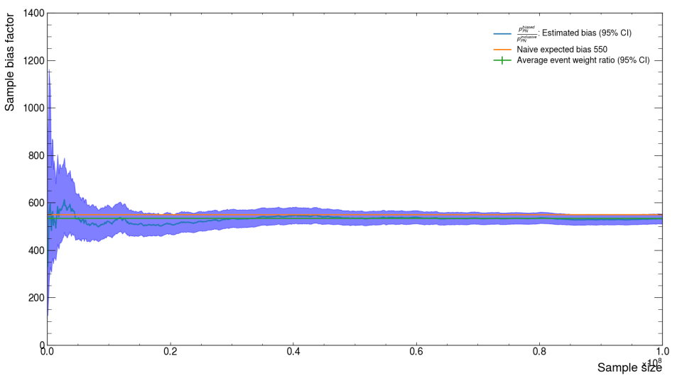
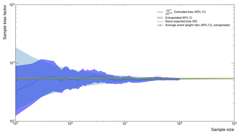
For example, a very common sample is the so-called "Ecal PN" sample where we bias and filter for a high-energy photon to be produced in the target and then have a photon-nuclear interaction in the Ecal mimicking our missing momentum signal. We can use this sample (along with an inclusive sample of the same size) to directly calculuate \(C\) with \(M/N\) and compare that value to our two estimators. Up to a sample size \(N\) of 1e8 (\(10^8\) both options for estimating \(C\) look okay (first image), but we can extrapolate out another order of magnitude and observe that only the second option \(W\) stays within the CI (second image).

Photon-Nuclear Re-sampling

Often we want to not only require there to be a photon-nuclear interaction in the Ecal, but we also want that photon-nuclear interaction to produce a specific type of interaction (usually specific types of particles and/or how energetic those particles are) -- known as the "event topology".

In order to support this style of sample generation, ldmx-sw is able to be configured such that when the PN interaction is happening, it is repeatedly re-sampled until the configured event topology is produced and then the simulation continues. The estimate \(W\) ends up being a slight over-estimate for samples produced via this more complicated process. Specifically, a "Kaon" sample where there is not an explicit biasing of the photon-nuclear interaction but the photon-nuclear interaction is re-sampled until kaons are produced already shows difference between the "true" value for \(C\) and our two short-hand estimates from before (image below).

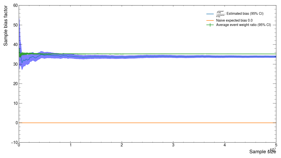
The overly-simple naive expected bias \(B\) is wrong because there is no biasing, but the average event weight ratio estimate \(W\) is also wrong in this case because the current (ldmx-sw v4.5.2) implementation of the re-sampling procedure updates the event weights incorrectly. Issue #1858 documents what we believe is incorrect and a path forward to fixing it. In the meantime, just remember that if you are using this configuration of the simulation, the estimate for the EoT explained above will be slighly higher than the "true" EoT. You can repeat this experiment on a medium sample size (here 5e7 = 50M events) where an inclusive sample can be produced to calculate \(C\) directly.